Modeling

As previously stated, exponential functions and logarithmic functions are used to model countless read-world phenomena. These functions are invaluable to science and engineering as we are able to model and manipulate the models to make predictions and solve problems.

Exponential Growth and Decay

For many exponential models, we use the general form $y = A_0e^{kt}$ where $A_0$ is equal to the value at time zero, $e$ is Euler's constant, and $k$ is a constant that determines the rate of growth or decay. If the value of $k$ is positive, the model represents exponential growth. If the value of $k$ is negative, the model represents exponential decay.

The function $y = A_0e^{kt}$ is a general function with the following characteristics:

1. It is a one-to-one function.
2. The horizontal asymptote is $y = 0$.
3. The domain is $(-\infty, \infty)$ and the range is $(0, \infty)$.
4. There is no $x$-intercept but there is a $y$-intercept at $(0, A_0)$.
5. The function is increasing if $k > 0$ and decreasing if $k < 0$.

Half-Life

One common application of exponential decay is the concept of half-life which is the length of time it takes an exponentially decaying quantity to decrease to half of its initial value. Every radioactive isotope has a half-life and the process describing the exponential decay of a radioactive isotope is called radioactive decay.

To find the half-life of a substance, we can set $y = \frac{1}{2}A_0$ in the general exponential model to get the equation $\frac{1}{2}A_0 = A_0e^{kt}$. We set $y$ to $\frac{1}{2}A_0$ because we are looking for the time it takes for the quantity to decrease to half of its initial value. The formula is derived as follows...

$$\begin{array}{llllllllll} \frac{1}{2}A_0 &=& A_0e^{kt} \\[3pt] \frac{1}{2} &=& e^{kt} \\[3pt] \ln(\frac{1}{2}) &=& \ln(e^{kt}) \\[3pt] \ln(\frac{1}{2}) &=& kt \\[3pt] \ln(2^{-1}) &=& kt \\[3pt] -\ln(2) &=& kt \\[3pt] \frac{-\ln(2)}{k} &=& t \\[3pt] \end{array}$$

We can solve for $t = \frac{-\ln(2)}{k}$ to find the half-life of the substance. We could also find the decay constant $k$ through $k = \frac{-\ln(2)}{t}$ by rearranging the formula.

$\underline{Example}$

The half-life of plutonium-244 is 80,000,000 years. Find a function that gives the amount of plutonium-244 remaining as a function of time $t$, measured in years.

Let's begin with the general exponential model and build from there...

$$\begin{array}{llllllllll} A &=& A_0e^{kt} \\ 0.5A_0 &=& A_0e^{80,000,000k} \\ 0.5 &=& e^{80,000,000k} \\ \ln(0.5) &=& 80,000,000k \\ k &=& \frac{\ln(0.5)}{80,000,000} \\ k &\approx& -8.66 \times 10^{-9} \\ \end{array}$$

The decay rate is $k \approx -8.66 \times 10^{-9}$. The function that gives the amount of plutonium-244 remaining as a function of time $t$ is $A \approx A_0e^{-8.66 \times 10^{-9}t}$.

note

The formula $t = \frac{-\ln(2)}{k}$ shows that half-life depends only on the decay constant $k$ and not on the initial quantity $A_0$.

The formula also shows that since $t$ is positive, the decay constant $k$ must be negative.

Radiocarbon Dating

Radiocarbon dating is a method used to calculate the approximate date a plant or animal died. This is possible through carbon-14 which is a radioactive isotope of carbon that has a half-life of $5,730$ years. It occurs in small quantities in the carbon dioxide we breathe. Most of the carbon on Earth is carbon-12, which has an atomic weight of $12$ and is not radioactive. Scientists have determined the ratio of carbon-14 to carbon-12 in the atmosphere and use this information to determine the age of organic materials.

As long as a plant or animal is alive, the ratio of the two isotopes of carbon in its body is close to the ratio in the atmosphere. When it dies, the carbon-14 in its body decays and is not replaced. By comparing the ratio of carbon-14 to carbon-12 in a decaying sample to the known ratio in the atmosphere, the date the plant or animal died can be approximated.

Since the half-life of carbon-14 is $5,730$ years, the formula for the amount of carbon-14 remaining after $t$ years is $A \approx A_0e^{(-\ln(2) / 5730)t}$ or $A \approx A_0e^{-0.000121t}$. The decay rate of carbon-14 was determined using the formula $k = \frac{-\ln(2)}{t}$.

From the equation, $A \approx A_0e^{-0.000121t}$, we know the ratio of the percentage of carbon-14 in the object we are dating to the initial amount of carbon-14 in the object when it was formed is $r = \frac{A}{A_0} = e^{-0.000121t}$. We solve this equation for $t$, to get $t = \frac{-\ln(r)}{0.000121}$ which is the formula used to calculate the age of the object.

$\underline{Example}$

A bone fragment is found that contains $20\%$ of its original carbon-14. To the nearest year, how old is the bone?

Using the formula $t = \frac{-\ln(r)}{0.000121}$, we can calculate the age of the bone.

We need to find the value of $r$ first which can be found through $r = \frac{A}{A_0}$. The value of $A$ is $20\%$ of the original amount of carbon-14, so $A = 0.20A_0$. This gives us $r = \frac{0.20A_0}{A_0} = 0.20$.

Substituting $r = 0.20$ into the formula $t = \frac{-\ln(r)}{0.000121}$, we get $t = \frac{-\ln(0.20)}{0.000121} \approx 13,301$ years.

The bone is approximately $13,301$ years old.

Doubling Time

The opposite of half-life is doubling time which is the time it takes for an exponentially growing quantity to double in value. Unlike, half-life and radiocarbon dating, the value of $k$ is positive for doubling time because we have exponential growth.

To find the doubling time of a quantity, we can set $y = 2A_0$ in the general exponential model to get the equation $2A_0 = A_0e^{kt}$. We set $y$ to $2A_0$ because we are looking for the time it takes for the quantity to double its initial value. The formula is derived as follows...

$$\begin{array}{llllllllll} 2A_0 &=& A_0e^{kt} \\[3pt] 2 &=& e^{kt} \\[3pt] \ln(2) &=& kt \\[3pt] \frac{\ln(2)}{k} &=& t \\[3pt] \end{array}$$

We can solve for $t = \frac{\ln(2)}{k}$ to find the doubling time of the substance. We could also find the growth constant $k$ through $k = \frac{\ln(2)}{t}$ by rearranging the formula.

$\underline{Example}$

According to Moore's Law, the doubling time for the number of transistors that can be put onto a computer chip is approximately $2$ years. Give a function that describes this behavior.

We need to find the growth constant $k$ first which can be found through $k = \frac{\ln(2)}{t}$. The doubling time is $2$ years, so $t = 2$. This gives us $k = \frac{\ln(2)}{2}$.

Substituting for $k = \frac{\ln(2)}{2}$ into the general exponential model, we get $y = A_0e^{\frac{\ln(2)}{2}t}$.

The function that describes the behavior is $y = A_0e^{\frac{\ln(2)}{2}t}$.

Newton's Law of Cooling

Newton's Law of Cooling states that the rate at which an object cools is proportional to the difference in temperature between the object and the object's surroundings. This means the temperature of an object will exponentially approach the temperature of its surroundings and it will level off as it gets closer to the surrounding temperature.

Unless the room temperature is zero, this will correspond to a vertical shift of the generic exponential function. The temperature of an object, $T$, in surrounding air with temperature $T_s$ will behave according to the formula $T(t) = Ae^{kt} + T_s$ where $t$ is time, $A$ is the difference between the initial temperature of the object and the surroundings, and $k$ is a constant that determines the continuous rate of cooling of the object.

Given a set of conditions, we can apply the Newton's Law of Cooling by...

1. Setting $T_s$ equal to the y-coordinate of the horizontal asymptote (the surrounding temperature or ambient temperature).
2. Substituting the given values into the continuous growth formula $T(t) = Ae^{kt} + T_s$ to find the parameters $A$ and $k$.
3. Substitute in the desired time to find the temperature of the object at that time.

$\underline{Example}$

A pitcher of water at $40$ degrees Fahrenheit is placed into a $70$ degree room. One hour later, the temperature has risen to $45$ degrees. How long will it take for the temperature to rise to $60$ degrees?

Due to the fact that the surrounding temperature is $70$ degrees, the pitcher of water will approach $70$ degrees as time goes on. The formula for the temperature of the water is $T(t) = Ae^{kt} + 70$.

We can use the fact that the initial temperature of the water is $40$ degrees to find the value of $A$...

$$\begin{array}{llllllllll} T(t) &=& Ae^{kt} + 70 \\ 40 &=& Ae^{k(0)} + 70 \\ 40 &=& Ae^0 + 70 \\ 40 &=& A(1) + 70 \\ A &=& -30 \\ \end{array}$$

We can use the fact that $A = -30$ and the fact that the temperature of the water is $45$ degrees after one hour to find the value of $k$...

$$\begin{array}{llllllllll} T(t) &=& -30e^{kt} + 70 \\ 45 &=& -30e^{k(1)} + 70 \\ 45 &=& -30e^k + 70 \\ -25 &=& -30e^k \\ \frac{5}{6} &=& e^k \\ k &=& \ln(\frac{5}{6}) \\ \end{array}$$

With the value of $A$ and $k$, we can model the temperature of the water as $T(t) = -30e^{\ln(\frac{5}{6})t} + 70$. We can use this model to find the time it takes for the temperature to rise to $60$ degrees by setting $T(t) = 60$ and solving for $t...

$$\begin{array}{llllllllll} T(t) &=& -30e^{\ln(\frac{5}{6})t} + 70 \\ 60 &=& -30e^{\ln(\frac{5}{6})t} + 70 \\ -10 &=& -30e^{\ln(\frac{5}{6})t} \\ \frac{1}{3} &=& e^{\ln(\frac{5}{6})t} \\ \ln(\frac{1}{3}) &=& \ln(\frac{5}{6})t \\ t &=& \frac{\ln(1 / 3)}{\ln(5 / 6)} \\ t &\approx& 6.026 \\ \end{array}$$

The temperature of the water will rise to $60$ degrees after approximately $6.026$ hours.

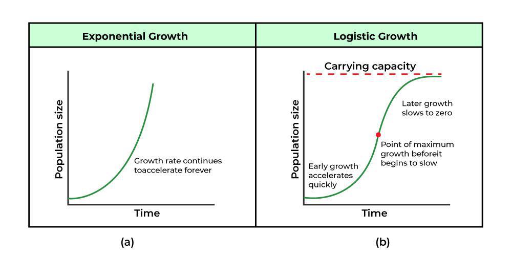
Logistic Growth

Exponential growth typically cannot continue indefinetly and so while exponential models may be useful in the short term, they tend to fall apart the longer they continue. Eventually, an exponential model must begin to approach some limiting value forcing the growth to slow down.

To achieve this, we use a logistic growth model which is approximately exponential at first, but it has a reduced rate of growth as the output approaches the model's upper bound, which is called the carrying capacity. The logistic growth model is $f(t) = \frac{c}{1 + ae^{-bt}}$ where $\frac{c}{1 + a}$ is the initial value, $c$ is the carrying capacity or limiting value, and $b$ is a constant determined by the rate of growth.

Fig. 1 - Logistic Growth Model

note

Given the logistic growth model $f(t) = \frac{c}{1 + ae^{-bt}}$. The initial value of population is $(0, \frac{c}{1 + a})$, the carrying capacity is $y = c$, and the point of maximum growth is $(\frac{\ln(a)}{b}, \frac{c}{2})$.

Models in Natural Base

Powers and logarithms of any base can be used in modeling, but the two most common bases are $10$ and $e$. It is important to note that in science and mathematics, the natural base $e$ is often preffered and so if we have a model in a different base, we typically convert it to the natural base.

Given a model with the form $y = ab^x$, we can change it to the form $y = A_0e^{kx}$ by...

1. Rewriting $y = ab^x$ as $y = ae^{ln(b^x)}$.
2. Using the power rule of logarithms, we can rewrite $y$ as $y = ae^{xln(b)} = ae^{ln(b)x}$.
3. Noting that $a = A_0$ and $k = ln(b)$, we can rewrite the model as $y = A_0e^{kx}$.

$\underline{Example}$

Change the function $y = 3(0.5)^x$ to one having $e$ as the base.

We can rewrite $y = 3(0.5)^x$ as $y = 3e^{\ln(0.5^x)}$.

Using the power rule of logarithms, we can rewrite $y$ as $y = 3e^{x\ln(0.5)} = 3e^{\ln(0.5)x}$.

Noting that $A_0 = 3$ and $k = \ln(0.5)$, we can rewrite the model as $y = 3e^{\ln(0.5)x}$.

The function with $e$ as the base is $y = 3e^{\ln(0.5)x}$.

Choosing Appropriate Models

When choosing models to represent data, we often use three kinds of functions: linear, exponential, and logarithmic. If the data lies on a straight line or seems to lie approximately along a straight line, a linear model may be best. If the data is non-linear, we often consider an exponential or logarithmic model. It must be noted that other models, such as quadratic, may also be considered.

When choosing between an exponential and logarithmic model, we look at the concavity of the data which is the way the data curves. If we draw a line between two data points, and most of the data between those two points lies above that line, we say the curve is concave down. The shape of a concave down curve is similar to a bowl that bends downwards and therefore cannot hold water. On the other hand, if most of the data between two points lies below the line, we say the curve is concave up. The shape of a concave up curve is similar to a bowl that bends upwards and therefore can hold water.

In most common cases, an exponential curve is always concave up, and a logarithmic curve is always concave down. Finally, a logistic curve changes concavity. It starts out concave yp and then changes to concave down beyond a certain point, called a point of inflection.