Graphing Exponential Functions

Exponential functions are used for many real-world applications in the sciences and business and they give us a method for making predictions. However, being able to make predictions off equations is not always enough. Being able to graph these functions can give us a visual representation of the data which is a powerful tool allowing us to arrive at more insightful conclusions.

Graphing

In order to graph exponential functions, we need to be able to graph the parent function $f(x) = b^x$ where $b > 0$ and $b \neq 1$. This parent function has the following characteristics which are useful to note when graphing...

1. It is a one-to-one function
2. There is a horizontal asymptote at $y = 0$
3. The domain is $(-\infty, \infty)$ and the range is $(0, \infty)$
4. There is no $x$-intercept but there is a $y$-intercept at $(0, 1)$
5. The graph is increasing if $b > 1$ and decreasing if $b < 1$

Noting all these properties, we can graph an exponential function of the form $f(x) = b^x$ by...

1. Creating a table of points.
2. Plotting at least $3$ points from the table, including the $y$-intercept $(0, 1)$.
3. Drawing a smooth curve through the points.
4. Stating the domain, range, and horizontal asymptote.

$\underline{Example}$

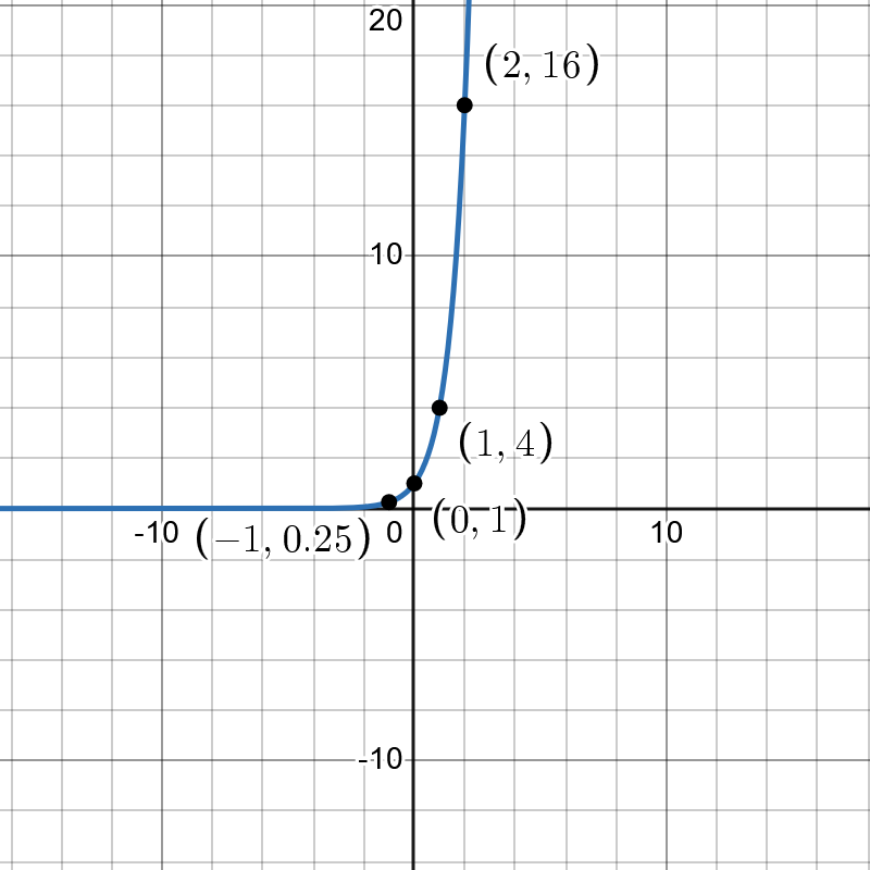
Sketch the graph of $f(x) = 4^x$. State the domain, range, and asymptote.

The first step is to create a table of points.

x	-1	0	1	2	3	4
y	0.25	1	4	16	64	256

Using the table, we want to plot at least $3$ points including the $y$-intercept. After that we should draw a smooth curve through the points.

Fig. 1 - Graph of Parent Function

All functions of the form $f(x) = b^x$ have the same domain, range, and horizontal asymptote. The domain is $(-\infty, \infty)$, the range is $(0, \infty)$ and the horizontal asymptote is $y = 0$.

note

For any exponential function of the form $f(x) = ab^x$, we call the base the constant ratio because as the input increases by $1$, the output value will be the product of the base and the previous output, regardless of the value of $a$. For example, if $f(x) = 2^x$ and $f(2) = 4$ then $f(3) = f(2) * b = 4 * 2 = 8$. This is useful when creating tables for graphing.

Transformations

We can take the parent function $f(x) = b^x$ and apply transformations to get any exponential function of the form $f(x) = ab^x$. This means with the ability to graph the parent function, we can graph any exponential function.

Vertical Shift

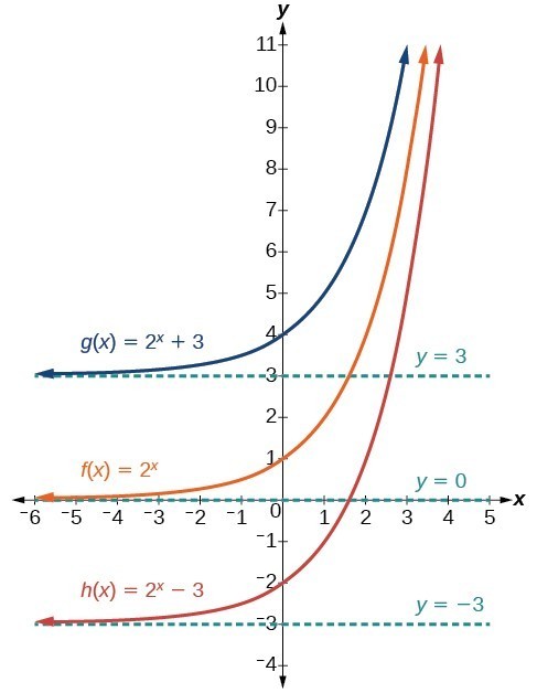
The first transformation occurs when we add a constant $d$ to the parent function $f(x) = b^x$, giving us $f(x) = b^x + d$. This shifts the graph vertically by $d$ units in the same direction as the sign of $d$.

Fig. 2 - Vertical Shift

When we perform a vertical shift, the new properties are...

1. The domain $(-\infty, \infty)$ remains the same.
2. The range is shifted by $d$ units and so the new range is $(d, \infty)$.
3. The horizontal asymptote shifts by $d$ units and so the new asymptote is $y = d$.
4. The $y$-intercept shifts by $d$ units and so the new $y$-intercept is $(0, 1 + d)$.

Horizontal Shift

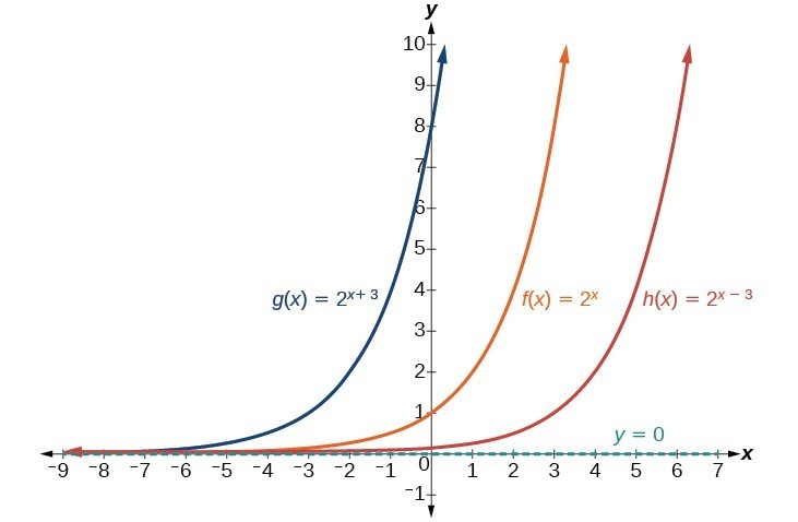
The second transformation occurs when we add a constant $c$ to the input of the parent function $f(x) = b^x$, giving us $f(x) = b^{x + c}$. This shifts the graph horizontally by $c$ units in the opposite direction of the sign of $c$.

Fig. 3 - Horizontal Shift

When we perform a vertical and horizontal shift, we get the equation of the form $f(x) = b^{x + c} + d$ where the new properties are...

1. The domain $(-\infty, \infty)$ remains the same.
2. The range is shifted by $d$ units and so the new range is $(d, \infty)$.
3. The horizontal asymptote shifts by $d$ units and so the new asymptote is $y = d$.
4. The $y$-intercept changes to $(0, b^c + d)$.

Stretch and Compression

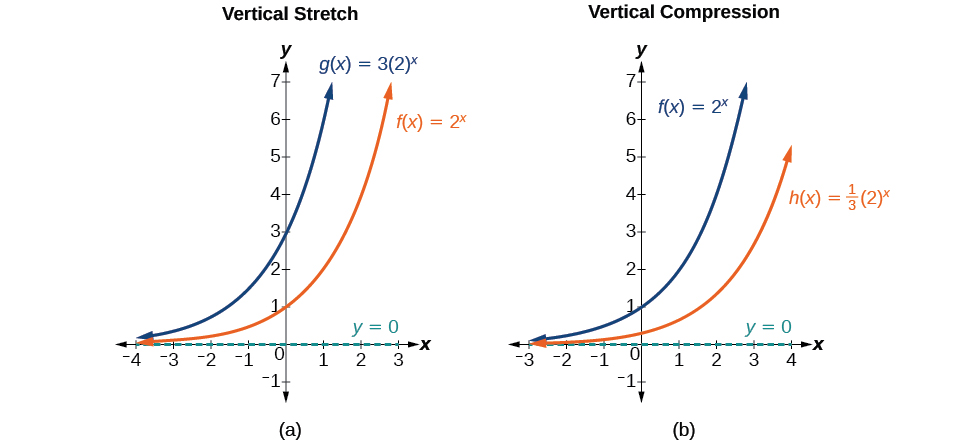
We can also stretch or compress the graph of the parent function by multiplying the parent function by a constant $a$, giving us $f(x) = ab^x$. If $|a| > 1$, the graph is stretched vertically by a factor of $a$ and if $|a| < 1$, the graph is compressed vertically by a factor of $a$.

Fig. 4 - Stretch and Compression

When we perform a stretch or compression, the new properties are...

1. The domain $(-\infty, \infty)$ remains the same.
2. The range $(0, \infty)$ remains the same.
3. The horizontal asymptote $y = 0$ remains the same.
4. The $y$-intercept changes to $(0, a)$.

Reflection

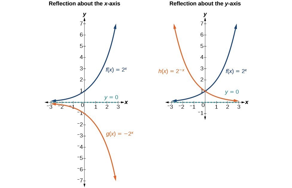
We can also reflect the graph of the parent function about the $x$-axis and the $y$-axis by multiplying the parent function by a negative constant.

To reflect about the $x$-axis, we use the function $f(x) = -b^x$ and it has the following properties...

1. The domain $(-\infty, \infty)$ remains the same.
2. The range is reflected about the $x$-axis and so the new range is $(-\infty, 0)$.
3. The horizontal asymptote is $y = 0$ and remains the same.
4. The $y$-intercept is $(0, -1)$.

To reflect about the $y$-axis, we use the function $f(x) = b^{-x} = (\frac{1}{b})^x$ and the properties stay the same as the parent function. Nothing changes except the graph is reflected about the $y$-axis.

Fig. 5 - Reflection

General Function

A translation of an exponential function has the form $f(x) = ab^{x + c} + d$ where the parent function, $y = b^x$, $b > 1$, is shifted horizontally $c$ units to the left, shifted vertically $d$ units, stretched vertically by a factor of $|a|$ if $|a| > 0$, compressed vertically by a factor of $|a|$ if $|a| < 1$, and reflected about the $x$-axis if $a < 0$.

$\underline{Example}$

Write the equation where $f(x) = e^x$ is compressed vertically by a factor of $\frac{1}{3}$, reflected about the $x$-axis, and then shifted down $2$ units. Graph the function and state the horizontal asymptote, the domain, the range, and the $y$-intercept.

Firstly, the equation is compressed vertically by a factor of $\frac{1}{3}$ so $a = \frac{1}{3}$. The function is then reflected about the $x$-axis so $a < 0$ which means $a = -\frac{1}{3}$. Finally, the function is shifted down $2$ units so $d = -2$. Putting everything together, we get the equation $f(x) = -\frac{1}{3}e^x - 2$.

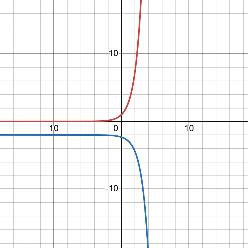
We can graph the function $f(x) = e^x$ and then transform it to get the graph of $f(x) = -\frac{1}{3}e^x - 2$.

Fig. 5 - Parent Function (Red) and Transformed Function (Blue)

The horizontal asymptote is $y = -2$ because the function is shifted down $2$ units. The domain is $(-\infty, \infty)$. Next, the range is $(-\infty, -2)$ because the function is shifted down $2$ units and reflected about the $x$-axis. Finally, the $y$-intercept is $(0, a + d) = (0, -\frac{1}{3} - 2) = (0, -\frac{7}{3})$ because of the vertical compression and the vertical shift.