Linear Functions

A linear function is a function with a constant rate of change. This is a polynomial with a degree of $1$.

The function notation for lienar functions is $f(x) = mx + b$ where $x$ is the input value, $m$ is the rate of change, and $b$ is the initial value of the dependent variable. Note that this function notation comes from the linear equation form which is $y = mx + b$.

Rate of Change

We can intrepret the slope as the rate of change of the function which is the change in the output values per unit of the input value. So given a function $f$, we can obtain the rate of change using the formula: $m = \frac{f(x_2) - f(x_1)}{x_2 - x_1}$. This means to obtain the rate of change, we only need two points $(x_1, f(x_1))$ and $(x_2, f(x_2))$ from the function $f$.

The function $f$ is an increasing function if $m > 0$, a decreasing function if $m < 0$ and a constant function if $m = 0$. The graph of an increasing function slants upwards from left to right. Vice versa, the graph of a decreasing function slants downwards from left to right. Finally, a constant function means the graph is a horizontal line.

Evaluation

If we have the slope (which can be found using two points) and any point, we can find the equation of a line using the point-slope form: $y - y_1 = m(x - x_1)$. We can rewrite the equation after in slope-intercept form in order to put it in function notation.

If we have the y-intercept or starting value instead, we can just write it in slope-intercept form and then in function notation form.

$\underline{Example}$

If $f(x)$ is a linear function, with $f(2) = -11$ and $f(4) = -25$, write an equation for the function in slope-intercept form.

$m = \frac{f(x_2) - f(x_1)}{x_2 - x_1} = \frac{(-25) - (-11)}{4 - 2} = \frac{-14}{2} = -7$

$y - y_1 = m(x - x_1)$

$y + 11 = -7(x - 2)$

$y + 11 = -7x + 14$

$y = -7x + 3$

$f(x) = -7x + 3$

Modeling

For any real world problem, we can model a linear function $f$ if we are given the initial value and rate of change. Once we have determined these two values, we substitute $b$ for the initial value and $m$ for the rate of change in $f(x) = mx + b$. After this, we often may need to solve for $f(c)$ which we can do by substituting $x = c$ and evaluating using it.

$\underline{Example}$

A new plant food was introduced to a young tree to test its effect on the height of the tree. The set of relations: $\{(0, 12.5), (2, 13.5), (4, 14.5), (8, 16.5), (12, 18.5)\}$ shows the height of the tree, in feet, $x$ months since the measurements began. Write a linear function $H(x)$, where $x$ is the number of months since the start of the experiment. Also predict the height of the tree in $20$ months.

$m = \frac{f(x_2) - f(x_1)}{x_2 - x_1} = \frac{13.5 - 12.5}{2 - 0} = \frac{1}{2}$

$H(x) = mx + b = 0.5x + 12.5$ where $12.5$ is the initial value.

$H(20) = 0.5(20) + 12.5 = 10 + 12.5 = 22.5$

$H(x) = 0.5x + 12.5$ and in $20$ months the tree will be $22.5$ feet.

Intercepts

Finally, to find the $x$-intercept of a linear function, we substitute $f(x) = 0$ and then solve for $x$.

$\underline{Example}$

Find the $x$-intercept of $f(x) = \frac{1}{4}x - 4$.

$0 = \frac{1}{4}x - 4$

$4 = \frac{1}{4}x$

$x = 16$

$x$-intercept: $(16, 0)$

Graphing

The graph of a linear function is a straight line. So, given at least two points, we can plot them on the grid and then draw a straight line through the points to get the graph of any linear function.

$\underline{Example}$

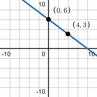
Graph $f(x) = -\frac{3}{4}x + 6$ by plotting points.

$f(0) = -\frac{3}{4}(0) + 6 = 0 + 6 = 6$

$f(4) = -\frac{3}{4}(4) + 6 = -3 + 6 = 3$

We can plot $(0, 6)$ and $(4, 3)$ and draw a straight line between them to get the graph of $f(x) = -\frac{3}{4}x + 6$.

Fig. 1 - Graph of f(x)

Using Rise over Run

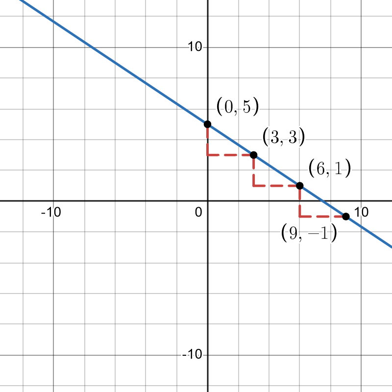
Given the function $f(x) = mx + b$, $b$ is the y-intercept of the graph which means it indicates the point $(0, b)$ which we can plot onto the grid. We can then use the fact that $m = \frac{\text{rise}}{\text{run}}$ to plot the rest of the graph. We move $\text{rise}$ units upwards and then $\text{run}$ units to the right to plot our next point. We connect these points using a straight line after.

$\underline{Example}$

Graph $f(x) = -\frac{2}{3}x + 5$ using the $y$-intercept and slope.

We graph $(0, 5)$ and then use rise over run to get the rest of the graph.

Fig. 2 - Graph of f(x)

Using Transformations

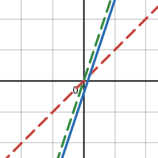
We can graph $f(x) = x$ and then vertically stretch or compress the graph by a factor of $m$. After this, we can shift the graph up or down $b$ units.

$\underline{Example}$

Graph $f(x) = 3x - 2$ using transformations.

Let the graph $f(x) = x$ be represented by the red dashed line. After vertically stretching by $3$, we get the green dashed line. Finally, we shift this graph down by $2$ to get our final graph.

Fig. 3 - Graph of f(x)

Function from Graphs

Finally, we can work backwards by using a graph to get the equation of the function. We first need to identify the $y$-intercept of the equation to get the value of $b$. After this we choose two points and use the slope formula to find the value of $m$. Finally, we can substitute $m$ and $b$ into the slope-intercept form to find the function of the line.

Horizontal and Vertical Lines

There are two special cases of straight line graphs: horizontal and vertical lines. A horizontal line is a line defined by an equation in the form $f(x) = b$ and has the slope $m = 0$. No matter the input value, the output value will stay the same. On the other hand, a vertical line is a line defined by an equation in the form $x = a$ and has an undefined slope. A vertical line is not a function as there are an infinite number of outputs for one input.

Parallel and Perpendicular

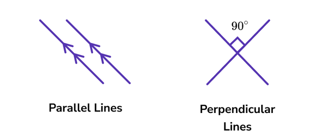
Two lines are parallel lines if they do not intersect and this happens if the slopes of the lines are the same. In mathematical terms, the functions $f(x) = m_1x + b_1$ and $g(x) = m_2x+b_2$ are parallel if and only if $m_1 = m_2$ and $b_1 \neq b_2$. If both $m_1 = m_2$ and $b_1 = b_2$, then the lines coincide and coincident lines are the same line.

Two lines are perpendicular lines if they intersect to form a right angle. In mathematical terms, the function $f(x) = m_1x + b_1$ and $g(x) = m_2x + b_2$ are perpendicular if and only if $m_1m_2 = -1$, so $m_2 = -\frac{1}{m_1}$.

Fig. 4 - Parallel and Perpendicular Lines