Graphing Logarithmic Functions

Logarithmic functions are used to model various real life situations and being able to graph them is invaluable as it allows us to visualize the function in order to analyze and predict trends.

Domain and Range

The domain of an exponential function of the form $y = b^x$ for any real number $x$ where $b > 0$ and $b \neq 1$ is $(-\infty, \infty)$. The range of this function is $(0, \infty)$. Now, given that logarithmic functions are inverses of exponential functions, the domain of a logarithmic function in the form of $y = \log_b(x)$ is $(0, \infty)$ and the range is $(-\infty, \infty)$.

When we applied certain transformations like vertical shift to the parent exponential function, the range of $y = b^x$ changed. Similarly, applying certain transformations to the parent function $y = \log_b(x)$ can change the domain. The domain of a logarithmic function consists only of positive real numbers and so, given a logarithmic function, we can identify the domain by setting up an inequality showing the argument of log greater than zero. We can then solve for $x$ and write the resulting domain in interval notation.

$\underline{Example}$

What is the domain of $f(x) = \log(x - 5) + 2$?

The argument of log is $x - 5$, we ignore the $2$ as it is outside the log. This gives us the inequality $x - 5 > 0$.

We can solve for $x$ by adding $5$ to both sides of $x - 5 > 0$ giving us $x > 5$.

Rewriting the domain in interval notation gives us $(5, \infty)$.

Graphing

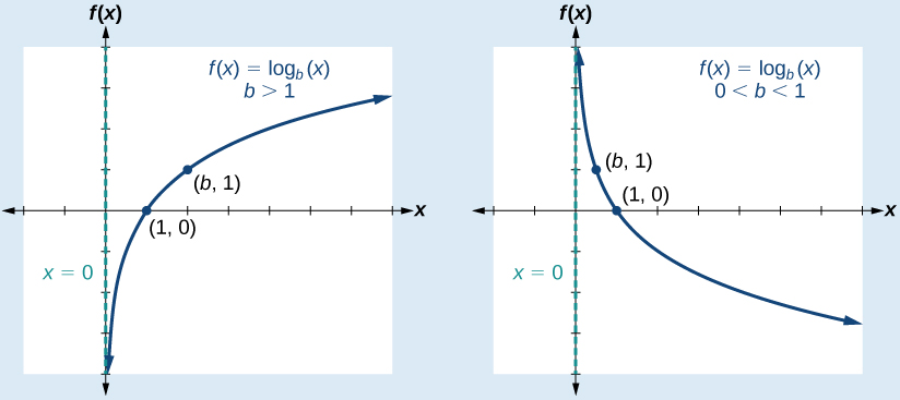
For any real number $x$ and constant $b > 0$ where $b \neq 1$, we get the following characteristics in the graph of $f(x) = \log_b(x)$...

1. It is a one-to-one function.
2. The domain is $(0, \infty)$ and the range is $(-\infty, \infty)$.
3. The $x$-intercept is $(1, 0)$ and there is no $$y-intercept.
4. A key point is $(b, 1)$.
5. The graph is increasing if $b > 1$ and decreasing if $0 < b < 1$.

Fig. 1 - Parent Logarithmic Function

Given a logarithmic function with the form $f(x) = \log_b(x)$, we can graph the function using the following steps...

1. Draw and label the vertical asymptote, $x = 0$.
2. Plot the $x$-intercept, $(1, 0)$.
3. Plot the key point $(b, 1)$.
4. Draw a smooth curve through the points.
5. State the domain, $(0, \infty)$, the range, $(-\infty, \infty)$, and the vertical asymptote, $x = 0$.

$\underline{Example}$

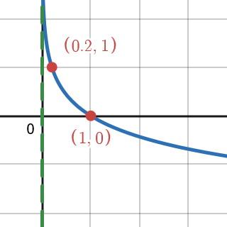
Graph $f(x) = \log_{\frac{1}{5}}(x)$. State the domain, range, and asymptote.

We can plot the points $(1, 0)$ and $(\frac{1}{5}, 1)$ and draw a smooth curve through those points. When drawing the curve, we will make sure to get close to $x = 0$ but never have our curve touch or cross it.

Fig. 2 - Graph of Example

The domain is $(0, \infty)$, the range is $(-\infty, \infty)$ and there is a vertical asymptote at $x = 0$.

Horizontal Shift

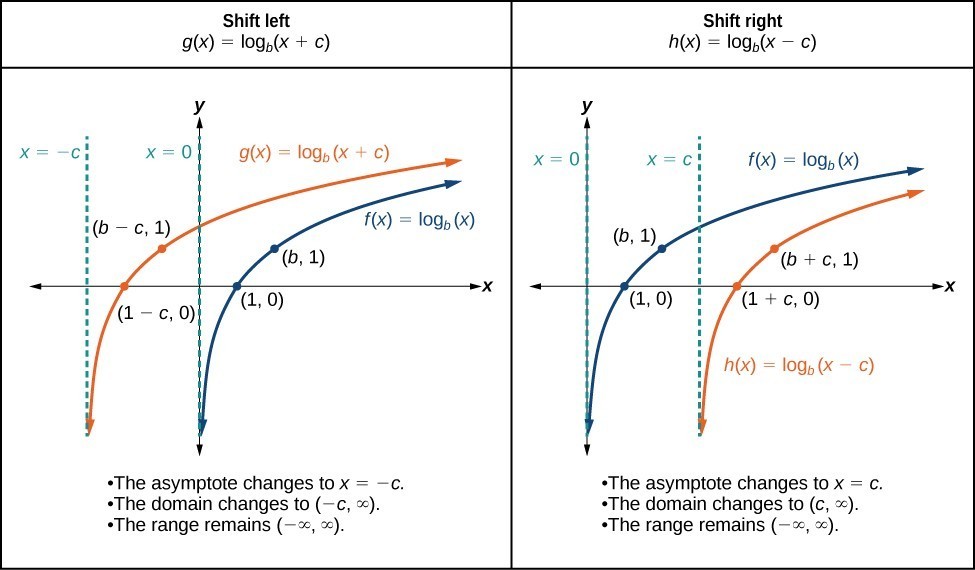
We can shift the parent function $c$ units horizontally using the function $f(x) = \log_b(x + c)$. If $c > 0$ then we shift $c$ units to the left and if $c < 0$, we shift $c$ units to the right. When we apply a horizontal shift, the vertical asymptote becomes $x = -c$, the domain becomes $(-c, \infty)$ and the range stays the same as $(-\infty, \infty)$.

Fig. 3 - Horizontal Shift

Vertical Shift

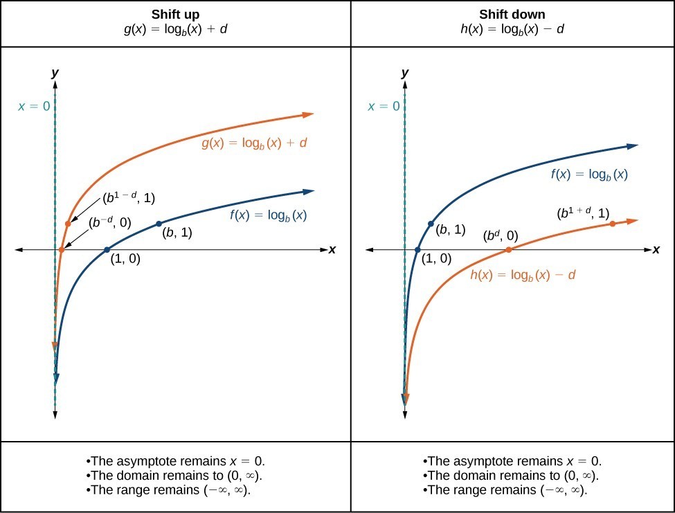
We can shift the parent function $d$ units vertically using the function $f(x) = \log_b(x) + d$. If $d > 0$ then we shift $d$ units up and if $d < 0$, we shift $d$ units down. When we apply a vertical shift, the vertical asymptote, domain, and range stay the same. This means the vertical asymptote is $x = 0$, the domain is $(0, \infty)$ and the range is $(-\infty, \infty)$.

Fig. 4 - Vertical Shift

Stretches and Compressions

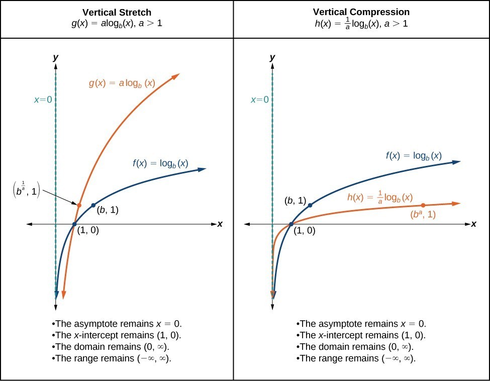
Given a positive constant $a$ where $a \neq 1$, we can stretch and compress the function using $f(x) = a\log_b(x)$. If $a > 1$ then we are stretching the parent function vertically by a factor of $a$ and if $0 < a < 1$ then we are compressing the parent function vertically by a factor of $a$. Doing this transformation does not change any of the properties of the parent function.

Fig. 5 - Stretch and Compress

Reflections

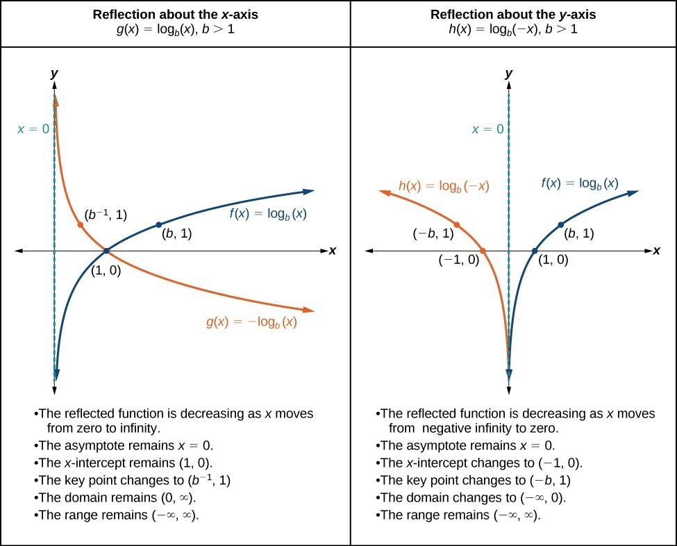
When the parent function is multiplied by $-1$ meaning $-f(x)$ or $f(x) = -\log_b(x)$, then the result is a reflection about the $x$-axis. The reflected function's vertical asymptote, domain, and range remains the same which means the vertical asymptote is $x = 0$, the domain is $(0, \infty)$ and the range is $(-\infty, \infty)$. However, the key point does change to $(b^{-1}, 1)$ and the reflected function changes directions as $x$ approaches $\infty$.

On the other hand, when the input of the parent function is multiplied by $-1$ meaning $f(-x)$ or $f(x) = \log_b(-x)$, then the result is a reflection about the $y$-axis. In this case, the vertical asymptote remains the same as $x = 0$ and the range remains the same as $(-\infty, \infty)$. The new $x$-intercept is $(-1, 0)$, the key point is now $(-b, 1)$ and the domain is now $(-\infty, 0)$.

Fig. 6 - Reflection

note

Due to the fact that exponential functions and logarithm functions are inverse functions, the parent functions are reflections of each other about $y = x$.

General Equation

All translations of the parent logarithmic function, $y = \log_b(x)$, has the form $f(x) = a\log_b(x + c) + d$ where $b > 1$. The constant $a$ denotes stretching or compressing, $c$ denotes the horizontal shift, and $d$ denotes the vertical shift. If $a < 0$ then there is a reflection about the $x$-axis and if $f(x) = \log(-x)$ then there is a reflection about the $y$-axis.

We can graph any logarithmic function by graphing the parent function and then translating it based on the constants found in the function. After this we can state the domain, range, and asymptote based on how they were altered through the translations.

$\underline{Example}$

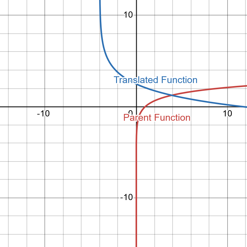
Graph the function of $f(x) = -2\log_3(x + 4) + 5$. State the domain, range, and vertical asymptote.

The parent function is $f(x) = \log_3(x)$ because the base is $3$. The graph has additional constants which are $a = -2$, $c = 4$, and $d = 5$. Through these constants we can denote that we are stretching the parent function by a scale of $2$, shifting it to the left $4$ units and down $5$ units. Finally, due to the fact that $a < 0$, we are reflecting about the $x$-axis.

Fig. 7 - Example Function

Due to the fact that we shifted $4$ units to the left, our new vertical asymptote is $x = -4$ and the new domain is $(-4, \infty)$. The range stays the same as $(-\infty, \infty)$.