Graphing Polynomial Functions

We are able to analyze polynomial equations through algebraic manipulation like factoring to find the zeros. However, another way to analyze polynomial functions is through their graphs which can sometimes make it easier to arrive at insights than with algebraic manipulation.

Degrees and Turning Points

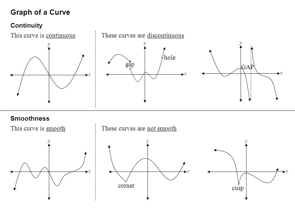
All graphs of polynomials of degree $2$ or more have graphs that are smooth curves meaning they have no sharp corners. These graphs are also continuous meaning they have no breaks.

Fig. 1 - Continuity and Smoothness

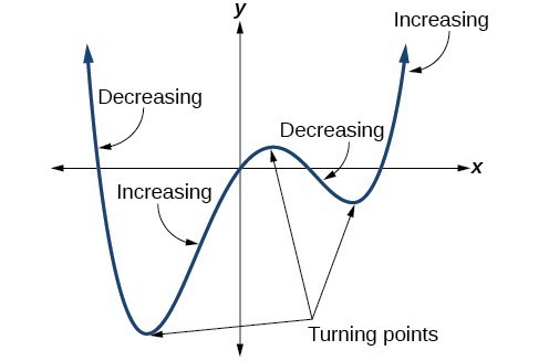
Even though these graphs have no sharp corner, they still transition between increasing to decreasing and decreasing to increasing. A turning point is a point of the graph where the graph changes from increasing to decreasing or decreasing to increasing. Note that a polynomial of degree $n$ will have at most $n - 1$ turning points.

Fig. 2 - Turning Points

Finding Zeros and Multiplicity

Given $f$ which is a polynomial function, then the zeros of $f$ are all the $x$-values for which $f(x) = 0$. The zeros can then be used to plot the $x$-intercepts of a polynomial graph.

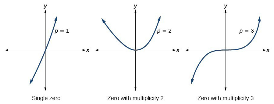
Graphs can end up having many $x$-intercepts but the graph can behave differently between those intercepts. Sometimes, the graph will cross over the horizontal axis at an intercept or sometimes it will just touch the horizontal axis. The behavior of these $x$-intercepts are not random and can be analyzed through multiplicity which is the number of times a given factor appears in the factored form of a polynomial function. In other words if a polynomial function contains a factor of the form $(x - h)^p$, the behavior near the $x$-intercept $h$ is determined by the power $p$. We can state that $x = h$ is a zero of multiplicity $p$.

1. If the graph crosses the $x$-axis at $x = a$ and appears almost linear at the intercept, then the multiplicity of $a$ is $1$.
2. If the graph touches the $x$ axis at $x = a$ and bounces off the axis, then the multiplicity of $a$ is even. For each increasing even power, the graph will appear flatter as it approaches and leaves the $x$-axis.
3. If the graph crosses the $x$-axis at $x = a$, then the multiplicity of $a$ is odd. For each increasing odd power, the graph will appear flatter as it approaches and leaves the $x$-axis.

Fig. 3 - Multiplicity

note

The sum of all the multiplicities for a function adds up to the degree of the function.

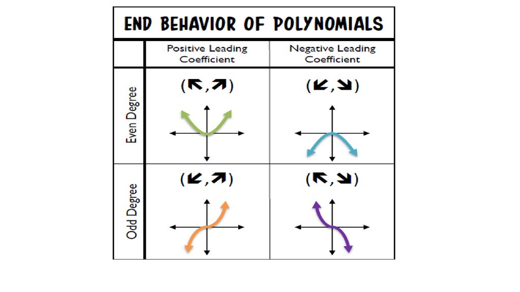
End Behavior

The end behavior of a polynomial function is the behavior of the graph as it approaches positive and negative infinity. All polynomial functions will either rise or fall as $x$ approaches infinity and negative infinity without bound. Note that the end behavior can be interpreted through the leading term of a polynomial function...

1. If the degree of the polynomial is even and the leading term is positive then $x$ increases without bound towards positive and negative infinity.
2. If the degree of the polynomial is even and the leading term is negative then $x$ decreases without bound towards positive and negative infinity.
3. If the degree of the polynomial is odd and the leading term is positive then $x$ increases without bound towards positive infinity and $x$ decreases without bound towards negative infinity.
4. If the degree of the polynomial is odd and the leading term is negative then $x$ decreases without bound towards positive infinity and $x$ increases without bound towards negative infinity.

Fig. 4 - End Behavior

Global and Local Extrema

A local minimum or local maximum is output at the lowest or highest point on the graph in an open interval around $x = a$. If a function has a local minimum at $a$, then $f(a) \leq f(x)$ for all $x$ in an open interval around $x = a$. Vice versa, if a function has a local maximum at $a$, then $f(a) \geq f(x)$ for all $x$ in an open interval around $x = a$.

A global minimum or global maximum is the output at the lowest or highest point of the function. If a function has a global minimum at $a$, then $f(a) \leq f(x)$ for all $x$. Vice versa, if a function has a global maximum at $a$, then $f(x) \geq f(x)$ for all $x$.

Fig. 5 - Minimum and Maximum

note

The local minimum and local maximum are sometimes referred to as the local extrema. On the other hand, the global minimum and global maximum are sometimes referred to as the global extrema.

Graphing

Given a polynomial function, we can sketch the graph using the following steps...

1. Find the intercepts.
2. Check for symmetry. If $f(-x) = f(x)$ then it is an even function and is symmetrical about the $y$-axis. On the other hand, if $f(-x) = -f(x)$ then it is an odd function and is symmetrical about the origin.
3. Use the multiplicities of the zeros to determine the behavior of the polynomial at the $x$-intercepts.
4. Determine the end behavior.
5. Use the end behavior and the behavior at the intercepts to sketch a graph.
6. Verify that the number of turning points does not exceed one less than the degree of the polynomial.

Writing Formulas

We can also work backwards and write formulas based on graphs. This is because we can take any polynomial of degree $p$ and use it's horizontal intercepts at $x = x_1, x_2, ..., x_n$ to get the factored form $f(x) = a(x - x_1)^{p_1}(x - x_2)^{p_2}...(x - x_n)^{p_n}$ where $p_i$ can be determined by the behavior of the graph at the corresponding intercept, and the stretch factor $a$ can be determined given a value other than the $x$-intercept. Using this logic we get the following steps...

1. Identify the $x$-intercepts of the graph to find the factors.
2. Examine the behavior the graph at the $x$-intercepts to determine the multiplicity of each factor.
3. Find the polynomial of least degree containing all the factors found in previous step.
4. Use any other point on the graph to determine the stretch factor.

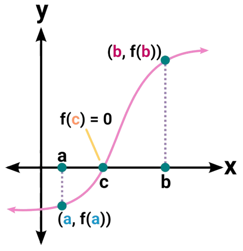
Intermediate Value Theorem

In some situations, we may know two points on a graph but not the zeros but we can still verify a zero exists using the Intermediate Value Theorem. Let $f$ be a polynomial function, then the theorem states that if $f(a)$ and $f(b)$ have opposite signs, then there exists at least one value $c$ between $a$ and $b$ for which $f(c) = 0$.

Fig. 6 - Intermediate Value Theorem