Other Trigonometric Functions

Besides cosine and sine, there are other trigonometric functions that are derived from them. These functions also have periodic properties and allow us to model real-world phenomena which makes it vital to be able to graph them as well.

Tangent Function

Recall that the tangent function is defined as $\tan \theta = \dfrac{\sin \theta}{\cos \theta}$ and it is periodic with a period of $\pi$. If we graph the tangent function on the interval $[-\dfrac{\pi}{2}, \dfrac{\pi}{2}]$, we are able to see the behavior of the graph on one complete cycle. So, to graph the tangent function, we can use the following table of values...

$x$	$-\dfrac{\pi}{2}$	$-\dfrac{\pi}{3}$	$-\dfrac{\pi}{4}$	$-\dfrac{\pi}{6}$	$0$	$\dfrac{\pi}{6}$	$\dfrac{\pi}{4}$	$\dfrac{\pi}{3}$	$\dfrac{\pi}{2}$
$\tan(x)$	$\text{undefined}$	$-\sqrt{3}$	$-1$	$-\dfrac{\sqrt{3}}{3}$	$0$	$\dfrac{\sqrt{3}}{3}$	$1$	$\sqrt{3}$	$\text{undefined}$

The graph of the tangent function is undefined at $x = -\dfrac{\pi}{2}$ and $x = \dfrac{\pi}{2}$ meaning they are vertical asymptotes. In order to graph the tangent function, we also need to consider the behavior of the graph at the points where the tangent function is undefined. This can be done by looking at the points near the asymptotes. For this case, lets look at points between $\dfrac{\pi}{3} \approx 1.05$ and $\dfrac{\pi}{2} \approx 1.57$...

$x$	$1.3$	$1.5$	$1.55$	$1.56$
$\tan(x)$	$3.6$	$14.1$	$48.1$	$92.6$

The value of the tangent function increases rapidly as $x$ approaches $\dfrac{\pi}{2}$. Lets also look at the points between $-\dfrac{\pi}{2} \approx -1.57$ and $-\dfrac{\pi}{3} \approx -1.05$ to see the behavior of the graph near the asymptote at $x = -\dfrac{\pi}{2}$...

$x$	$-1.3$	$-1.5$	$-1.55$	$-1.56$
$\tan(x)$	$-3.6$	$-14.1$	$-48.1$	$-92.6$

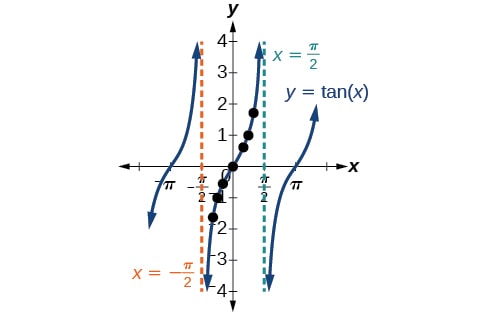
The value of the tangent function decreases rapidly as $x$ approaches $-\dfrac{\pi}{2}$. With all this information, we can now graph the tangent function...

Fig. 1 - Tangent Function

note

The tangent function is an odd function because sine is an odd function and cosine is an even function. This causes tangent to be odd because the tangent function is equivalent to the quotient of an odd function and an even function which always results in an odd function. In fact, any function that is the quotient of an odd function and an even function is an odd function.

General Equation

Similar to the sine and cosine functions, the tangent function can also be described by a general equation. The general equation of the tangent function is $y = A\tan(Bx - C) + D$ where $A$, $B$, $C$, and $D$ are all constants.

The features of the graph of $y = A\tan(Bx - C) + D$ are as follows...

• The stretching factor is $|A|$.
• The period is $\dfrac{\pi}{|B|}$.
• The domain is $x \neq \dfrac{C}{B} + \dfrac{\pi}{2}k$ where $k$ is an integer.
• The range is $(-\infty, \infty)$.
• The vertical asymptotes occur at $x = \dfrac{C}{B} + \dfrac{\pi}{2}k$ where $k$ is an odd integer.
• There is no horizontal asymptote.
• There is no amplitude.

Graphing Tangent

Given the function $y = A \tan(Bx - C) + D$, we can sketch the graph of one period using the following steps...

1. Verify the function is in the form $y = A \tan(Bx - C) + D$.
2. Identify the stretching/compressing factor, $|A|$.
3. Identify $B$ and use it to find the period, $P = \dfrac{\pi}{|B|}$.
4. Identify $C$ and use it to find the phase shift, $\dfrac{C}{B}$.
5. Sketch the vertical asymptotes, which occur at $x = \dfrac{C}{B} + \dfrac{\pi}{2|B|}k$ where $k$ is an odd integer.
6. For $AB > 0$, the graph approaches the left asymptote at negative output values and the right asymptote at positive output values. On the other hand, for $AB < 0$, the graph approaches the left asymptote at positive output values and the right asymptote at negative output values.
7. Obtain the reference points at $(\dfrac{P}{4}, A)$, $(0, 0)$, and $(-\dfrac{P}{4}, -A)$.
8. Shift the reference points to the right by $\dfrac{C}{B}$ and up by $D$.
9. Sketch the graph using the reference points and the asymptotes.

An example of graphing the tangent function is shown below...

$\underline{Example}$

Graph one period of the function $y = 2\tan(\pi x + \pi) - 1$.

The function is in the form $y = A\tan(Bx - C) + D$ so we are good to continue.

The stretching factor is $|A| = 2$.

The constant $B = \pi$ so the period is $P = \dfrac{\pi}{|B|} = \dfrac{\pi}{|\pi|} = 1$.

The constant $C = -\pi$ so the phase shift is $\dfrac{C}{B} = \dfrac{-\pi}{\pi} = -1$.

The vertical asymptotes occur at $x = \dfrac{C}{B} + \dfrac{\pi}{2|B|}k = -1 + \dfrac{\pi}{2(|\pi|)}k = -1 + \dfrac{1}{2}k$ where $k$ is an odd integer. Some of the vertical asymptotes are at $x = -1 + \dfrac{1}{2}(-1) = -1 - \dfrac{1}{2} = -\dfrac{3}{2}$ and $x = -1 + \dfrac{1}{2}(1) = -1 + \dfrac{1}{2} = -\dfrac{1}{2}$.

The constant $AB = 2(\pi) = 2\pi$ where $2\pi > 0$. This means the graph approaches the left asymptote at negative output values and the right asymptote at positive output values.

The reference points are at $(\dfrac{P}{4}, A) = (\dfrac{1}{4}, 2)$, $(0, 0)$, and $(-\dfrac{P}{4}, -A) = (-\dfrac{1}{4}, -2)$.

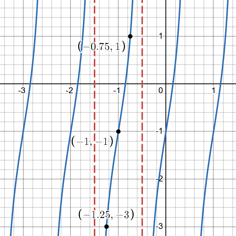
Shifting the reference points to the right by $\dfrac{C}{B} = -1$ and up by $D = -1$ gives us the points $(-\dfrac{3}{4}, 1)$, $(-1, -1)$, and $(-\dfrac{5}{4}, -3)$.

Using the reference points and the asymptotes, we can sketch the graph of the function...

Fig. 2 - Graph of Tangent Example

Secant Function

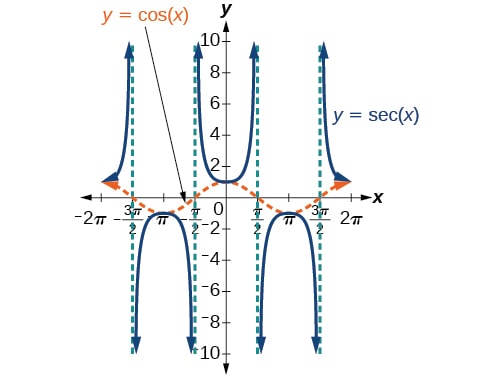
The secant function can also be defined as $\sec \theta = \dfrac{1}{\cos \theta}$. Considering the fact that the function is undefined when cosine is equal to $0$, the secant function has vertical asymptotes at $\dfrac{\pi}{2}$, $\dfrac{3\pi}{2}$, etc. Also note that since the cosine function will never be less than $-1$ or greater than $1$, the secant function will never be between $-1$ and $1$ as cosine is in the denominator.

Putting this all together, this gives us the graph of the secant function...

Fig. 3 - Secant Function

note

Since cosine is an even function, secant is also an even function. This is because the reciprocal of any even function is also an even function.

General Equation

The general equation of the secant function is $y = A\sec(Bx - C) + D$ where $A$, $B$, $C$, and $D$ are all constants.

The features of the graph of $y = A\sec(Bx - C) + D$ are as follows...

• The stretching factor is $|A|$.
• The period is $\dfrac{2\pi}{|B|}$.
• The domain is $x \neq \dfrac{C}{B} + \dfrac{\pi}{2|B|}k$, where $k$ is an odd integer.
• The range is $(-\infty, -|A| + D] \cup [|A| + D, \infty)$.
• The vertical asymptotes occur at $x = \dfrac{C}{B} + \dfrac{\pi}{2|B|}k$ where $k$ is an odd integer.
• There is no horizontal asymptote.
• There is no amplitude.

Graphing Secant

Given the function $y = A\sec(Bx - C) + D$, we can sketch the graph of one period using the following steps...

1. Verify the function is in the form $y = A\sec(Bx - C) + D$.
2. Identify the stretching/compressing factor, $|A|$.
3. Identify $B$ and use it to find the period, $P = \dfrac{2\pi}{|B|}$.
4. Identify $C$ and use it to find the phase shift, $\dfrac{C}{B}$.
5. Sketch the vertical asymptotes, which occur at $x = \dfrac{C}{B} + \dfrac{\pi}{2|B|}k$ where $k$ is an odd integer.
6. Sketch the graph of $y = A\cos(Bx - C) + D$.
7. Use the reciprocal relationship between $y = \cos x$ and $y = \sec x$ to sketch the graph.

$\underline{Example}$

Graph one period of $f(x) = -6\sec(4x + 2) - 8$.

The function is in the form $y = A\sec(Bx - C) + D$ so we are good to continue.

The stretching factor is $|A| = 6$.

The constant $B = 4$ so the period is $P = \dfrac{2\pi}{|B|} = \dfrac{2\pi}{4} = \dfrac{\pi}{2}$.

The constant $C = -2$ so the phase shift is $\dfrac{C}{B} = \dfrac{-2}{4} = -\dfrac{1}{2}$.

The vertical asymptotes occur at $x = \dfrac{C}{B} + \dfrac{\pi}{2|B|}k$ where $k$ is an odd integer. Some of the vertical asymptotes are at $x = -\dfrac{1}{2} + \dfrac{\pi}{8}(-1) = -\dfrac{1}{2} - \dfrac{\pi}{8}$ and $x = -\dfrac{1}{2} + \dfrac{\pi}{8}(1) = -\dfrac{1}{2} + \dfrac{\pi}{8}$.

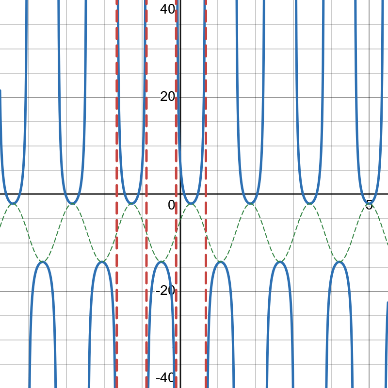
We can now graph the function using the recriprocal relationship between $y = \cos x$ and $y = \sec x$...

Fig. 4 - Graph of Secant Example

Cosecant Function

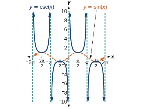
The cosecant function can also be defined as $\csc \theta = \dfrac{1}{\sin \theta}$. Similar to the secant function, the cosecant function is undefined when sine is equal to $0$ which gives us vertical asymptotes at $0$, $\pi$, $2\pi$, etc. Also, since the sine function will never be less than $-1$ or greater than $1$, the cosecant function will never be between $-1$ and $1$ as sine is in the denominator.

This gives us the graph of the cosecant function...

Fig. 5 - Cosecant Function

note

Since sine is an odd function, cosecant is also an odd function. This is because the reciprocal of any odd function is also an odd function.

General Equation

The general equation of the cosecant function is $y = A\csc(Bx - C) + D$ where $A$, $B$, $C$, and $D$ are all constants.

The features of the graph of $y = A\csc(Bx - C) + D$ are as follows...

• The stretching factor is $|A|$.
• The period is $\dfrac{2\pi}{|B|}$.
• The domain is $x \neq \dfrac{C}{B} + \dfrac{\pi}{|B|}k$, where $k$ is an integer.
• The range is $(-\infty, -|A| + D] \cup [|A| + D, \infty)$.
• The vertical asymptotes occur at $x = \dfrac{C}{B} + \dfrac{\pi}{|B|}k$ where $k$ is an integer.
• There is no horizontal asymptote.
• There is no amplitude.

Graphing Cosecant

Given the function $y = A\csc(Bx - C) + D$, we can sketch the graph of one period using the following steps...

1. Verify the function is in the form $y = A\csc(Bx - C) + D$.
2. Identify the stretching/compressing factor, $|A|$.
3. Identify $B$ and use it to find the period, $P = \dfrac{2\pi}{|B|}$.
4. Identify $C$ and use it to find the phase shift, $\dfrac{C}{B}$.
5. Sketch the vertical asymptotes, which occur at $x = \dfrac{C}{B} + \dfrac{\pi}{|B|}k$ where $k$ is an integer.
6. Sketch the graph of $y = A\sin(Bx - C) + D$.
7. Use the reciprocal relationship between $y = \sin x$ and $y = \csc x$ to sketch the graph.

$\underline{Example}$

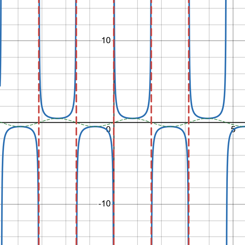
Graph one period of $f(x) = 0.5\csc(2x)$.

The function is in the form $y = A\csc(Bx - C) + D$ so we are good to continue.

The stretching factor is $|A| = 0.5$.

The constant $B = 2$ so the period is $P = \dfrac{2\pi}{|B|} = \dfrac{2\pi}{2} = \pi$.

The constant $C = 0$ so the phase shift is $\dfrac{C}{B} = \dfrac{0}{2} = 0$.

The vertical asymptotes occur at $x = \dfrac{C}{B} + \dfrac{\pi}{|B|}k = 0 + \dfrac{\pi}{2}(k)$ where $k$ is an integer. Some of the vertical asymptotes are at $x = -\pi$, $x = -\dfrac{\pi}{2}$, $x = 0$, $x = \dfrac{\pi}{2}$, and $x = \pi$.

We can now graph the function using the recriprocal relationship between $y = \sin x$ and $y = \csc x$...

Fig. 6 - Graph of Cosecant Example

Cotangent Function

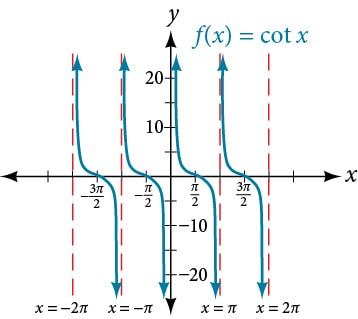
Finally, the cotangent function can be defined as $\cot \theta = \dfrac{1}{\tan \theta}$. Considering the fact that the function is undefined when tangent is equal to $0$, the cotangent function has vertical asymptotes at $0$, $\pi$, $2\pi$, etc. Also, since the output of the tangent function is all real numbers, the cotangent function will also have all real numbers as its output.

This gives us the graph of the cotangent function...

Fig. 7 - Cotangent Function

note

Since tangent is an odd function, cotangent is also an odd function. This is because the reciprocal of any odd function is also an odd function.

General Equation

The general equation of the cotangent function is $y = A\cot(Bx - C) + D$ where $A$, $B$, $C$, and $D$ are all constants.

The features of the graph of $y = A\cot(Bx - C) + D$ are as follows...

• The stretching factor is $|A|$.
• The period is $\dfrac{\pi}{|B|}$.
• The domain is $x \neq \dfrac{C}{B} + \dfrac{\pi}{|B|}k$, where $k$ is an integer.
• The range is $(-\infty, \infty)$.
• The vertical asymptotes occur at $x = \dfrac{C}{B} + \dfrac{\pi}{|B|}k$ where $k$ is an integer.
• There is no horizontal asymptote.
• There is no amplitude.

Graphing Cotangent

Given the function $y = A\cot(Bx - C) + D$, we can sketch the graph of one period using the following steps...

1. Verify the function is in the form $y = A\cot(Bx - C) + D$.
2. Identify the stretching/compressing factor, $|A|$.
3. Identify $B$ and use it to find the period, $P = \dfrac{\pi}{|B|}$.
4. Identify $C$ and use it to find the phase shift, $\dfrac{C}{B}$.
5. Sketch the vertical asymptotes, which occur at $x = \dfrac{C}{B} + \dfrac{\pi}{|B|}k$ where $k$ is an integer.
6. Sketch the graph of $y = A\tan(Bx - C) + D$.
7. Use the reciprocal relationship between $y = \tan x$ and $y = \cot x$ to sketch the graph.

$\underline{Example}$

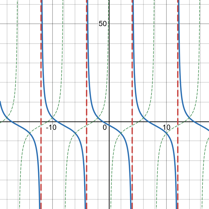
Sketch a graph of one period of the function $f(x) = 4\cot(\dfrac{\pi}{8}x - \dfrac{\pi}{2}) - 2$.

The function is in the form $y = A\cot(Bx - C) + D$ so we are good to continue.

The stretching factor is $|A| = 4$.

The constant $B = \dfrac{\pi}{8}$ so the period is $P = \dfrac{\pi}{|B|} = \dfrac{\pi}{\dfrac{\pi}{8}} = 8$.

The constant $C = \dfrac{\pi}{2}$ so the phase shift is $\dfrac{C}{B} = \dfrac{\dfrac{\pi}{2}}{\dfrac{\pi}{8}} = 4$.

The vertical asymptotes occur at $x = \dfrac{C}{B} + \dfrac{\pi}{|B|}k = 4 + 8k$ where $k$ is an integer. Some of the vertical asymptotes are at $x = 4 + 8(-1) = -4$, $x = 4 + 8(0) = 4$, $x = 4 + 8(1) = 12$, etc.

We can now graph the function using the recriprocal relationship between $y = \tan x$ and $y = \cot x$...

Fig. 8 - Graph of Cotangent Example