Graphing Polar Equations

Just as a rectangular equation such as $y = x^2$ describes the relationship between $x$ and $y$ on a Cartesian coordinate plane, a polar equation describes the relationship between $r$ and $\theta$ on a polar coordinate plane. In both of these systems, the equation is not the only way to represent the relationship because a graph can also be used. By graphing polar equations, we can visualize the relationship between $r$ and $\theta$ and better understand the behavior of the equations.

Testing Symmetry

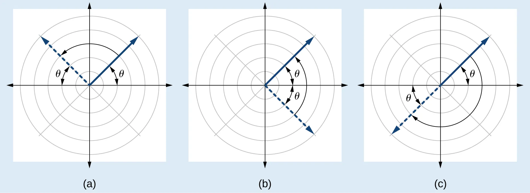
An equation of a graph is symmetric with respect to an axis if we can fold the graph along that axis and have both halves match up perfectly. For polar graphs, we typically test for three types of symmetry: symmetry about the polar axis (the horizontal axis), symmetry about the line $\theta = \dfrac{\pi}{2}$ (the vertical axis), and symmetry about the pole (the origin).

Fig. 1 - Types of Symmetry in Polar Graphs

After substituting the appropriate values into the equation, if we end up with an equivalent equation, then the graph is symmetric about that axis. The tests are as follows...

1. To test for symmetry about the polar axis, we replace $\left(r, \theta\right)$ with $\left(r, -\theta\right)$ in the equation.
2. To test for symmetry about the line $\theta = \dfrac{\pi}{2}$, we replace $\left(r, \theta\right)$ with $\left(-r, -\theta\right)$.
3. To test for symmetry about the pole, we replace $\left(r, \theta\right)$ with $\left(-r, \theta\right)$.

$\underline{Example}$

Test the equation for symmetry: $r = -2 \cos \theta$.

We can start by testing for symmetry about the polar axis by replacing $\left(r, \theta\right)$ with $\left(r, -\theta\right)$...

$$\begin{array}{ccccccccccccc} r &=& -2 \cos \theta \\[1em] r &=& -2 \cos \left(-\theta\right) \\[1em] r &=& -2 \cos \theta \\[1em] \end{array}$$

It is equivalent, so the graph is symmetric about the polar axis.

Next, we can test for symmetry about the line $\theta = \dfrac{\pi}{2}$ by replacing $\left(r, \theta\right)$ with $\left(-r, -\theta\right)$...

$$\begin{array}{ccccccccccccc} r &=& -2 \cos \theta \\[1em] -r &=& -2 \cos \left(-\theta\right) \\[1em] -r &=& -2 \cos \theta \\[1em] r &=& 2 \cos \theta \\[1em] \end{array}$$

It is not equivalent, so the graph is not symmetric about the line $\theta = \dfrac{\pi}{2}$.

Finally, we can test for symmetry about the pole by replacing $\left(r, \theta\right)$ with $\left(-r, \theta\right)$...

$$\begin{array}{ccccccccccccc} r &=& -2 \cos \theta \\[1em] -r &=& -2 \cos \theta \\[1em] r &=& 2 \cos \theta \\[1em] \end{array}$$

It is not equivalent, so the graph is not symmetric about the pole.

Therefore, the graph of the equation $r = -2 \cos \theta$ is symmetric about the polar axis only.

Graphing Polar Equations

To graph a polar equation, we can create a table of $\theta$ and $r$ values and then plot the points on a polar coordinate plane. However, we can use some strategies like properties of symmetry and identifying key values of $\theta$ and $r$ to make the process easier by requiring fewer points.

Identifying Zeros and Maxima

To find the zeros of a polar equation, we can set $r = 0$ and solve for $\theta$. On the other hand, to find the maxima, we substitute $\theta$ for a value that would result in the maximum value of the trigonometric function. For example, if the equation contains $\sin \theta$, we would substitute $\theta = \dfrac{\pi}{2}$ because $\sin \dfrac{\pi}{2} = 1$. On the contrary, if the equation contains $\cos \theta$, we would substitute $\theta = 0$ because $\cos 0 = 1$.

$\underline{Example}$

Graph the equation: $r = 2 \sin \theta$.

First, we can identify the properties of the equation like the type of symmetry and the zeros and maxima. After that, we can create a table of values and plot the points on a polar coordinate plane.

Let's begin by testing for symmetry for all three types...

$$\begin{array}{ccccccccccccc} r &=& 2 \sin \theta &&& r &=& 2 \sin \theta &&& r &=& 2 \sin \theta \\[1em] r &=& 2 \sin \left(-\theta\right) &&& -r &=& 2 \sin \left(-\theta\right) &&& -r &=& 2 \sin \theta \\[1em] r &=& -2 \sin \theta &&& -r &=& -2 \sin \theta &&& r &=& -2 \sin \theta \\[1em] &&&&& r &=& 2 \sin \theta &&&&& \\[1em] \end{array}$$

The graph is symmetric about the line $\theta = \dfrac{\pi}{2}$ only.

Next, we can find the zeros by setting $r = 0$ and solving for $\theta$...

$$\begin{array}{ccccccccccccc} r &=& 2 \sin \theta \\[1em] 0 &=& 2 \sin \theta \\[1em] \sin \theta &=& 0 \\[1em] \theta &=& 0, \pi, 2\pi, n\pi \\[1em] \end{array}$$

Finally, before creating a table of values, we can find the maximum by substituting $\theta = \dfrac{\pi}{2}$ because the equation contains $\sin \theta$ and $\sin \dfrac{\pi}{2} = 1$ which is the maximum value of the sine function...

$$\begin{array}{ccccccccccccc} r &=& 2 \sin \theta \\[1em] r &=& 2 \sin \left(\dfrac{\pi}{2}\right) \\[1em] r &=& 2 \left(1\right) \\[1em] r &=& 2 \\[1em] \end{array}$$

The maximum value of $r$ is 2 when $\theta = \dfrac{\pi}{2}$. So, the maxima is $\left(2, \dfrac{\pi}{2}\right)$.

Now that we have identified all the properties of the equation, we can create a table of values. We know that we can reflect points across the line $\theta = \dfrac{\pi}{2}$, so we only need to find points from $0$ to $\dfrac{\pi}{2}$. We can choose to find points at intervals of $\dfrac{\pi}{6}$...

$r$	$0$	$1$	$\sqrt{3}$	$2$
$\theta$	$0$	$\dfrac{\pi}{6}$	$\dfrac{\pi}{3}$	$\dfrac{\pi}{2}$

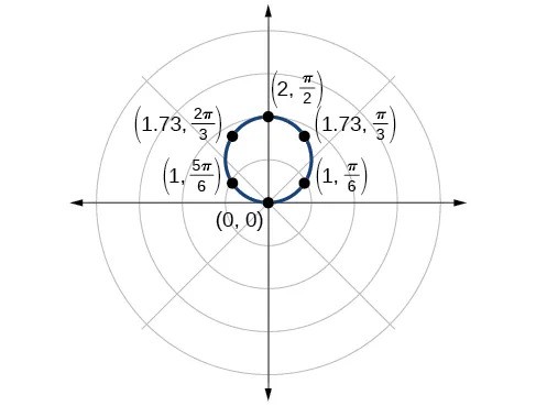
So, plotting the points gives us the following graph...

Fig. 2 - Example Polar Graph

Polar Curves

To be able to graph polar equations more easily, it helps to be familiar with the common types of curves that can be represented by polar equations. By recognizing the type of curve, we can use its properties to graph it more efficiently.

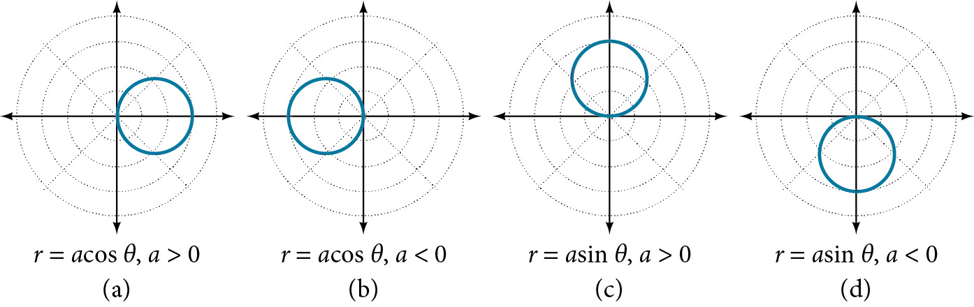
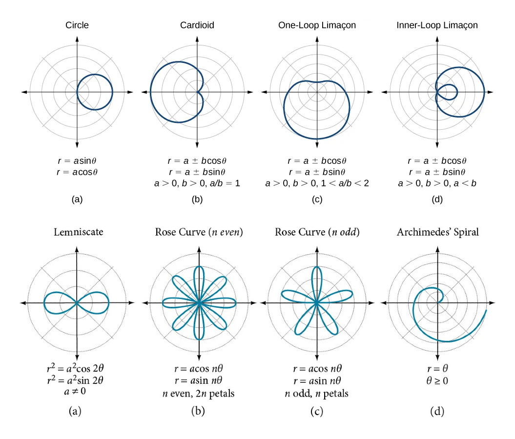
The most basic polar curve is the circle which are given by $r = a \cos \theta$ or $r = a \sin \theta$ where $a$ is the diameter of the circle or the distance from the pole to the farthest point on the circumference.

Fig. 3 - Polar Curve

note

For $r = a \cos \theta$, the center is $\left(\dfrac{a}{2}, 0\right)$ and for $r = a \sin \theta$, the center is $\left(\dfrac{a}{2}, \dfrac{\pi}{2}\right)$.

Cardioids

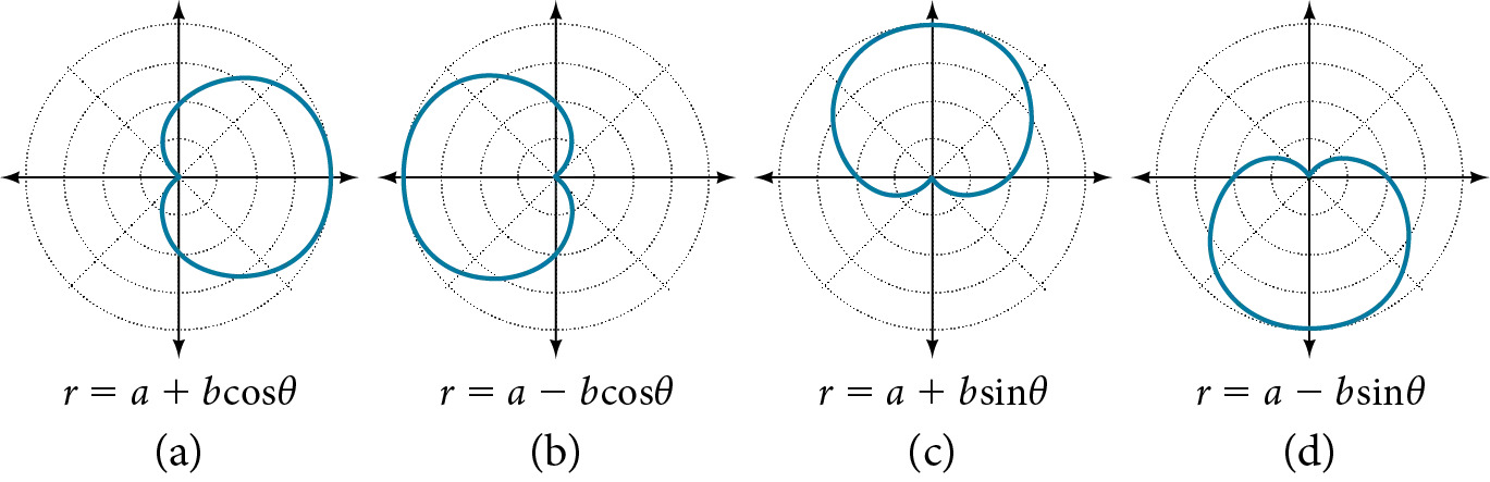
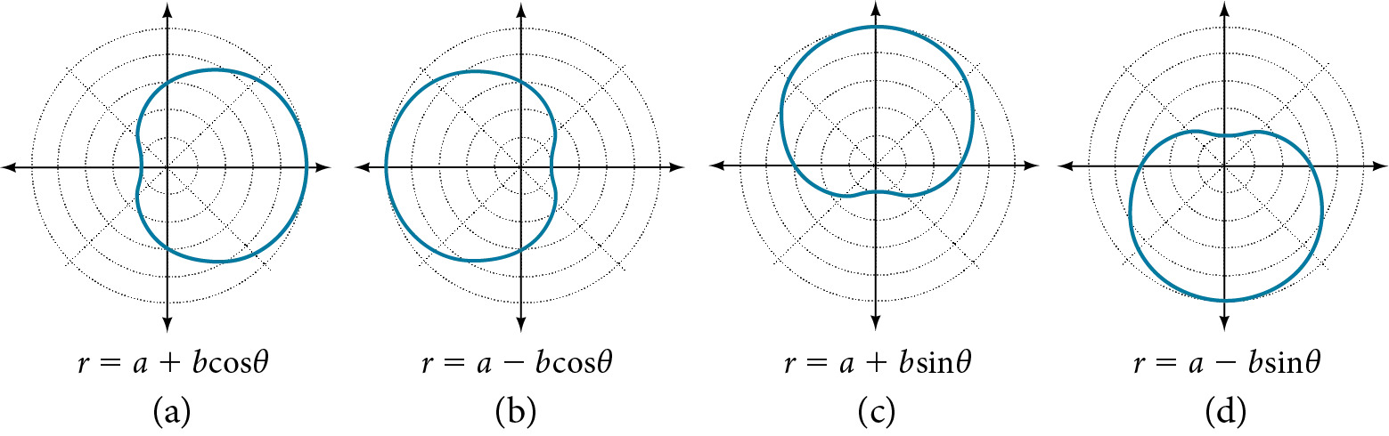
One of the classic polar curves is the cardioid which resembles a heart shape. The formulas that produce cardioids include $r = a \pm b \cos \theta$ and $r = a \pm b \sin \theta$ where $a > 0$, $b > 0$, and $\dfrac{a}{b} = 1$.

Fig. 4 - Cardioids

Limacons

Another classic polar curve is the limacon which is an old french word for "snail" which describes the shape of the curve.

One-loop limacons which are also refered to as dimpled limacons are given by the formulas $r = a \pm b \cos \theta$ and $r = a \pm b \sin \theta$ where $a > 0$, $b > 0$, and $1 < \dfrac{a}{b} < 2$.

Fig. 5 - One-Loop Limacons

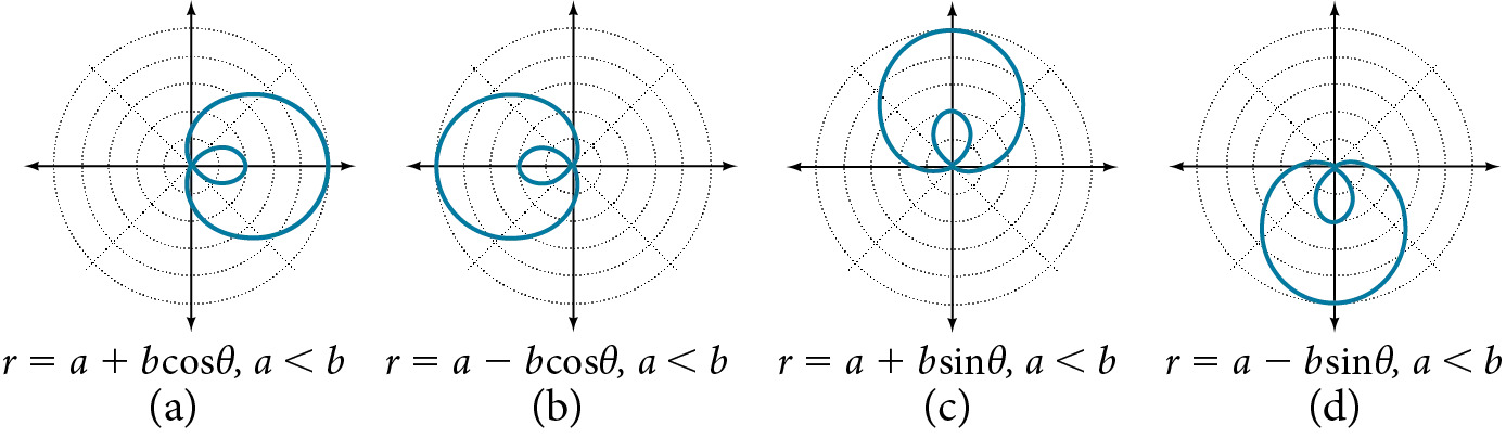
On the other hand, inner-loop limacons are given by the formulas $r = a \pm b \cos \theta$ and $r = a \pm b \sin \theta$ where $a > 0$, $b > 0$, and $a < b$. The graph of the inner-loop limacon passes through the pole twice where it is once for the outer loop and once for the inner loop.

Fig. 6 - Inner-Loop Limacons

note

Cardioids are a member of the limacon family where $\dfrac{a}{b} = 1$ and is the reason why we can see the similarities in the graphs.

Lemniscates

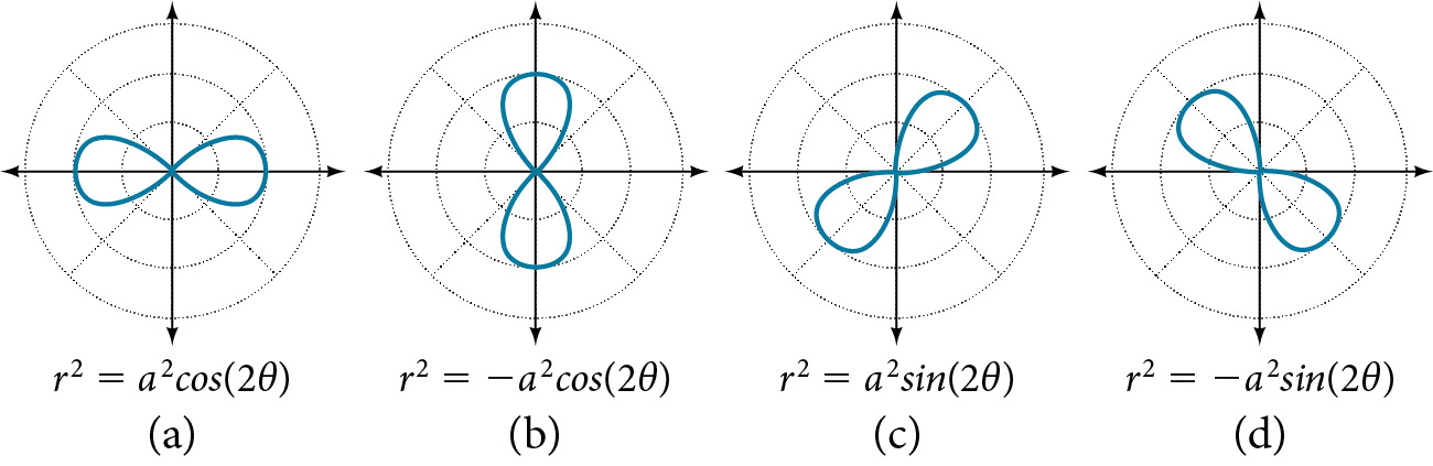
The lemniscate is another type of the classic polar curves which resembles a figure-eight or an infinity symbol. The formulas that produce lemniscates include $r^2 = a^2 \cos 2\theta$ and $r^2 = a^2 \sin 2\theta$ where $a \neq 0$.

Fig. 7 - Lemniscates

note

The formula $r^2 = a^2 \sin 2\theta$ produces a lemniscate that is symmetric with respect to the pole while the formula $r^2 = a^2 \cos 2\theta$ produces a lemniscate that is symmetric with respect to the line $\theta = \dfrac{\pi}{2}$ and the polar axis.

Rose Curves

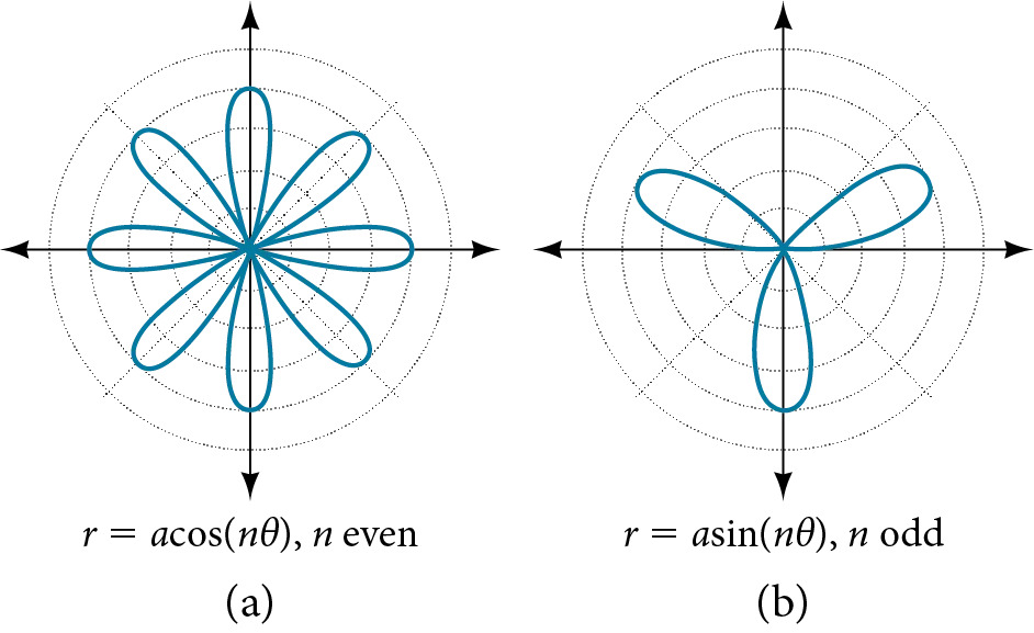
The next type of polar curve is the rose curve which produces a petal-like shape. This shape can be achieved by using the formulas $r = a \cos n\theta$ and $r = a \sin n\theta$ where $a \neq 0$. If $n$ is odd, then the rose curve will have $n$ petals. However, if $n$ is even, then the rose curve will have $2n$ petals.

Fig. 8 - Rose Curves

Archimedes Spiral

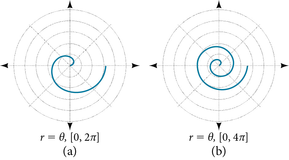
Finally, the Archimedes spiral is a polar curve given by $r = \theta$ where $\theta \geq 0$. For this curve, as $\theta$ increases, $r$ also increases at a constant rate in an never ending spiral that never intersects itself.

Fig. 9 - Archimedes Spiral

Summary

So, to summarize, here are the common types of polar curves along with their formulas and properties...

Fig. 10 - Summary of Polar Curves