Program Efficiency
Even though computers are getting faster every day, efficiency still plays a major factor because datasets that our programs run are growing just as fast. Simple solutions may not scale with large datasets which means the program could take extremely long to run.
Measuring Efficiency
To be able to choose effective algorithms, we need to have a way to calculate the efficiency of any algorithm we have.
One approach is to time an algorithm at the start a timer right before the algorithm starts and ends when the algorithm finishes running.
import time

# This simple algorithm converts celsius to fahrenheit
def c_to_f(c):
    return c * 9/5 + 32

# Starts the timer
start = time.clock()
# Runs the algorithm
c_to_f(1000)
# Gets the total runtime
end = timer.clock() - start

# Prints results
print("Total Runtime:", end)
Time is great because it varies based on what algorithm we test so it gives us a way to compare them. However, time varies between computers and is not predictable based on small inputs so it is difficult to create a relationship between inputs and time.
A better approach is to count operations and worry about how it grows as the program gets larger.
def fact_iter(arr):
    total = 1 # One Operation
    # Loops through the list
    for i in range(len(arr)):
        total += arr[i] # Size of Input Impacts Operations Here
    return total # One Operation
# With N being size, this takes N + 2 operations to complete
This approach is better because it is independent of what computer is running the program. It gives us a more abstract way to measure efficiency. However, we can improve this approach even further.
When we measure efficiency, we care about how the algorithm scales as the input grows. This means constant time operations that are not impacted by input size will not affect the scaling. For example, for the N + 2 operations, N is the size of the list and as the list grows, the 2 does not impact how the algorithm scales. We only care about the term that most impacts the efficiency which in this case is N.
Order of Growth
There are three ways we are look at efficiency. How well the algorithm performs in the best case, the average case, and the worst case. However, we should focus on worst case for efficiency first because we want to verify the algorithm works well even in the worst case scenario. We use the Big Oh Notation to measure an upper bound on the asymptotic growth (basically the worst case).
Like we declared above, we focus on the operations that change the most as the input size grows. The efficiency of the algorithm above was O(N) meaning it grows linearly.
Types of Growth
There are 6 types of growth terms we will find when measuring growth complexity (classes of growth)...
| Type | Growth Term |
|---|---|
| Constant | O(1) |
| Logarithmic | O(log n) |
| Linear | O(n) |
| Log Linear | O(n log n) |
| Polynomial | O(n^c) where c is a constant |
| Exponential | O(c^n) where c is a constant |
The table above is ordered from most efficient to least efficient growth complexities.
Constant
We get constant run time when the code does not depend on the size of the problem.
def arr_size(arr, arr2):
    return len(arr_size)
The example above runs one operation and returns the length of the list. Even if the list size grows, the function will still take the same number of operations to run so this is O(1).

Linear
We get linear run time when the algorithm has only a simple iteration or recursive element to it.
def linear_search(L, e):
    for i in range(len(L)):
        if e == L[i]:
            return True
    return False
This code looks for if the element e exists in the list L. In the worst case scenario, the element will not exist and that means this algorithm loops through the whole list once. This means this is O(n) because n is the size of the list and this is dependent on the size of the list.
def fact_recur(n):
    if n <= 1:
        return 1
    else:
        return n * fact_recur(n - 1)
This code is also O(n) because it only goes through the list once.

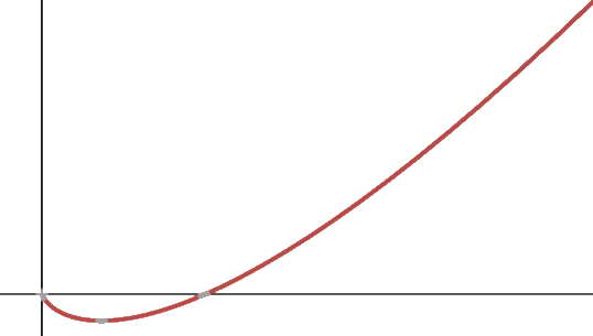
Polynomial
Polynomial complexity occurs when there are nested loops or recursive calls.
for i in range(n): # O(n)
    for j in range(n): # O(n)
        print('a')
# O(n) * O(n) = O(n^2)
This takes O(n^2) because it is a nested loop so everytime the first loop runs, the second loop runs once. If the nested loop was three layers deep then it would be O(n^3).
If the loop does not depend on the size of the list, then it has a constant runtime. This is O(n^2) because both loops in this nested loop depend on the size of the list.

Logarithmic
These are typically algorithms that reduce the problem in half each time through a process. An example of this is bisection search which takes a sorted list at looks for an element. It starts at the middle and checks if it is the element. If not it checks if the element is going to be in the upper half or lower half of the list because the list is sorted. In this fashion, it eliminates half the list during each iteration.
def bisect_search_helper(L, e, low, high):
    if high == low: # The whole list is checked
        return L[low] == e
    mid = (low + high) // 2 # Checks the current midpoint
    if L[mid] == e: # Checks if the element is found
        return True:
    elif L[mid] > e:
        if low == mid: # Makes sure end is not reached
            return False
        else:
            return bisect_search_helper(L, e, low, mid - 1) # Ignores higher half of list
    else:
        return bisect_search_helper(L, e, mid + 1, high) # Ignores lower half of list

def bisect_search(L, e):
    if len(L) == 0: # Ignores empty list
        return False
    else:
        return bisect_search_helper(L, e, 0, len(L) - 1)
This algorithm reduces the list in half each time it searches so it has an efficiency of O(log n).

Exponential
Exponential runtime typically occurs for algorithms that have multiple recursive calls at each level.
def fib_recur(n):
    if n == 0:
        return 0
    elif n == 1:
        return 1
    else:
        return fib_recur(n - 1) + fib_recur(n - 2)
For each level, the algorithm goes into two different recursive calls. So for each size, the amount of recursive calls double which is exponential. To show this we write that the efficiency is O(2^n) which signifies that it doubles as the input size increases.

Log Linear
Log Linear is a unique runtime that we will see in the next section with algorithms like merge sort. These algorithms are faster than polynomial algorithms but slower than linear ones.