Recursion and Dictionaries
Looping with for loops and while loops are iterative however, there are other ways to repeat items which could end up simplifying code even further. We call this other method recursion. Our lists and tuples are great ways to store large amounts of data however there are also more flexible options like dictionaries which may be better for some use cases.
Recursion
Recursion is the process of repeating items in a self-similar way where algorithmically it is a way to design solutions to problems by divide and conquer or decrease and conquer. On the other hand, semantically it is a programming technique where a function calls itself using a base case which is easy to solve and the other inputs given are able to be simplified.
For example, lets say we want a method to multiply two non negative numbers together using only addition.
# a * b = a + a + ... b times
def multiply(a, b):
    total = 0
    for i in range(b):
        total += a
    return a
This function uses a and loops through it b times to solve the problem. This would be an iterative approach but it can look cleaner using recursion. Let's say I want to do 2 * 5, another way we can look at it is (2 * 4) + 2. The (2 * 4) is a simplier version of the bigger problem and if we keep going down, we get to the simplist case where 2 * 0 = 0. This is our base case. The base case is the simplist form of the problem.
Now with recursion, you keep feeding a smaller problem back into your function until you get to the base case.
# a * b = a + (a * (b - 1))
def multiply(a, b):
    if b < 1:
        return 0
    return a + multiply(a, b - 1)
Let's trace this code which means go through it line by line to see what it is doing.
1. Let's give a = 3, b = 3 which should return 9.

2. First 3 < 1 is checked which is false.

3. We return 3 + multiply(3, 2). We can't return anything till we solve this smaller problem.

4. Now 2 < 1 is checked because b is now 2 and that returns false.

5. We return 3 + multiply(3, 1). We still cannot return anything and keep doing a smaller problem.

6. Now 1 < 1 is checked which is also false.

7. We return 3 + multiply(3, 0).

8. Now 0 < 1 is checked which is true!!! So 0 gets returned.

9. Now we now that multiply(3, 0) = 0 so multiply(3, 1) can return 3 + 0.

10. multiply(3, 2) returns 3 + 3 because multiply(3, 1) = 1.

11. multiply(3, 3) returns 3 + 6 because multiply(3, 2) = 6.

12. The final solution given is 9.
The multiply() function showed how to use recursion however, it wasn't a very practical use of recursion. One widely used case for recursion is solving for factorials.
Factorials
Factorials are numbers denoted by n! = n * (n - 1) * .... This means 3! = 3 * 2 * 1 and 5! = 5 * 4 * 3 * 2 * 1. Our base cases for factorials are 1! = 1 and 0! = 1.
It makes more sense to code factorials recursively than to do it iteratively because there is a clear way to divide up the problem to a smaller problem. Doing 3! = 3 * 2 * 1 but also 3! = 3 * 2!.
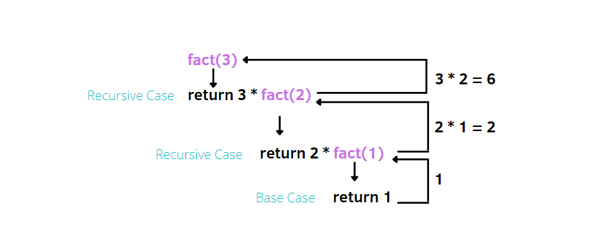
Each call is slowly building up the solution by solving a simplier version of the problem.
def fact(n):
    if n <= 1:
        return 1
    return n * fact(n - 1)
Recursion can make code look cleaner and simplier but it is important to note that may not be efficient from a computer's prespective because of all the different calls you are making on top of each other.
Scope
Scope plays a crucial factor in recursion because each recursive call to a function creates a new scope. This means any variable you bind in one function scope cannot be accessed by another function scope.
In the code for factorial, let's give a n of 5. The first function can see that n = 5 in its scope. When it calls the function again with n - 1. The new scope creates a brand new n with the value 4 and thats all it thinks n is. This way variables between each recursive call don't interfere with each other.
More Examples
Recursion can be a very abstract concept at the start. A few more examples can show the potential recursion has to writing cleaner, more understandable code.
We can use recursion for the fibonacci sequence. The sequence works by adding the previous two numbers to get a new number. So the first ten numbers in the sequence are 0, 1, 1, 2, 3, 5, 8, 13, 21, 34. To get a number like 21, we needed to add 8 and 13 which were the previous numbers to get that value.
This is a recursive problem because the new solution relies on simplier solutions. The function is f(n) = f(n - 1) + f(n - 2) where f(n - 1) and f(n - 2) are smaller problems to the bigger problem f(n). We also can say our base case is n <= 0 because the simpliest n is 0 which equals 0.
def fib(n):
    if n <= 0:
        return 0
    return fib(n - 1) + fib(n - 2)
Another example of recursion is finding is a string is a palidrome because the simpliest case you can get is a single letter or no letters. Every other size can check the first and last letters to see if they are the same and then remove them from the string. In this way we are slowly simplifying the problem to get to the answer.
def pali(word):
    # We have to remote all punctionation
    word = word.strip()

    # Base case
    if len(word) <= 1:
        return True

    # Checks last two letters
    if word[0] != word[-1]:
        return False

    # Shortens word and recursively checks
    return pali(word[1:-1])
As long as this call reaches the base case it is true because all the letters passed their checks. If at any point two letters are different, it will immediately exit.
Dictionaries
Dictionaries are another way to store data but with dictionaries we have more control over the indicies. With lists and tuples, we use zero-based indexing meaning we start counting by zero and to get a value, we specify its position in the list. With dictionaries, store them in no particular order, instead we do key-value pairs. Every unique key we create acts as the index to some value. The benefit being the key doesn't have to be integers only.
# Creates an empty dictionary
empty_dict = {}

# Creates a dictionary
# The key and value are seperated using a colon (:)
# Each pair is seperated by a comma (,)
grades = {'Ana':'B', 'John', 'A+'}
grades_num = {'Ana': 80, 'John': 99}

# The key can be almost anything
position = {1:"First", 2:"Second"}

# Access a value
print(grades['Ana']) # B

# Change a key value pair (Dictionaries are mutable)
grades['Ana'] = 'B+'
print(grades['Ana']) # B+

# You can check if a key exists
print('Ana' in grades) # True
print('Anastic' in grades) # False
print('A+' in grades) # False (Only key checks)

# Delete a pair
del grades['Ana']

# Get a list of all the keys
grades.keys()

# Get a list of all the values
grades.values()
As noted above that, dictionaries are mutable meaning they can be changed just like lists. However, it should also be noted that not all key types are valid. Any data type that is immutable can be used as a key. The final most important thing to note is that there is no order to dictionaries meaning pairs can be ordered randomly in memory.
Just to reiterate the point that even though dictionaries are mutable, keys must be immutable.
Recursion with Dictionaries
You can combine both recursion with dictionaries to improve the performance of recursion for problems like fibonacci.
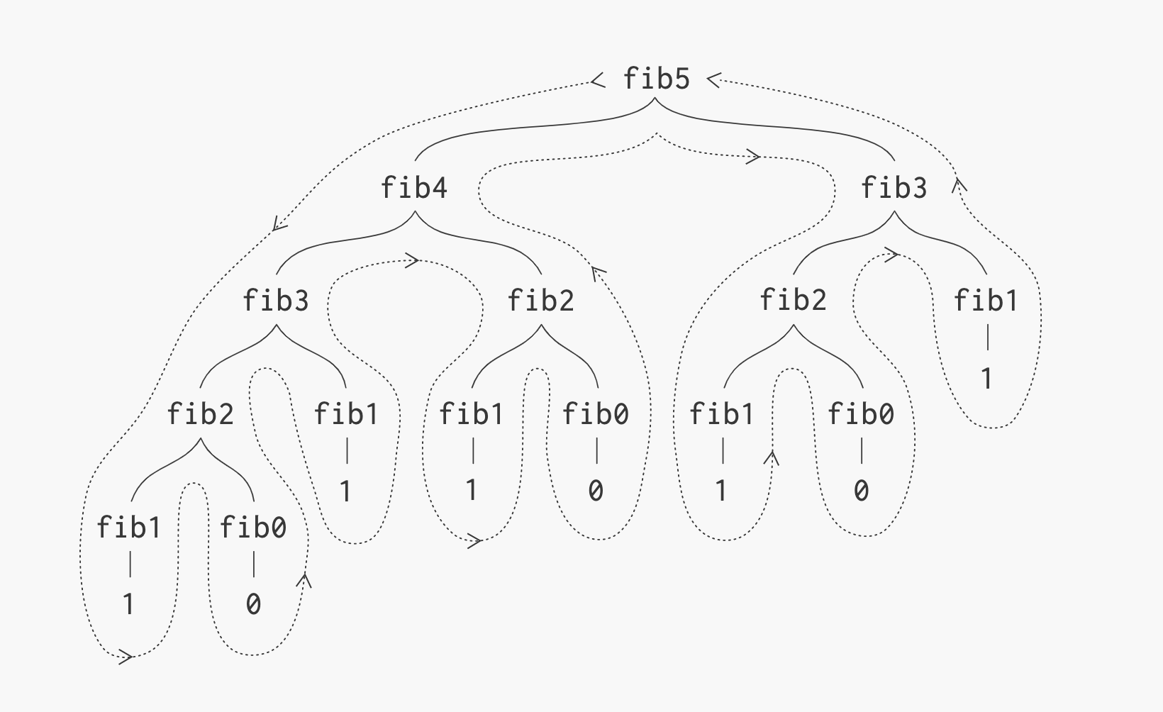
As seen here, if we recursively do the fibonacci sequence of 5, it recalculates fib(0), fib(1), fib(2) and so on many times. As our n gets bigger, the number of repeated calculations increases extremely fast. One way to solve this is to save results that are already computed in a dictionary so calculations do not have to occur multiple times. If we already know wat fib(3) is in this figure then we wouldn't need to calculate fib(2) and fib(1) again, we could just use the result we already stored.
# No saving (old fibonacci sequence)
def fib(n):
    # Use two base cases to slightly improve performance
    if n <= 0:
        return 0
    elif n == 1:
        return 1
    # Recursively calculate new values
    return fib(n - 1) + fib(n - 2)

# With saving
results = {}
def new_fib(n):
    # Checks if we already know the answer before calculating
    if n in results:
        # Returns stored answer
        return results[n]

    # Goes back to base case
    if n <= 0:
        return 0
    elif n == 1:
        return 1

    # Saves result after calculating for future use
    results[n] = new_fib(n - 1) + new_fib(n - 2)

    # Returns result
    return results[n]
The second method is called memoization which is the process of saving results to speed up programs. If we did something like fib(34) it would take 11,405,773 recursive calls to arrive at the answer but with new_fib(n) it only takes 65 because the results are saved.